Difference between revisions of "Sequential analysis"
(Importing text file) |
Ulf Rehmann (talk | contribs) m (MR/ZBL numbers added) |
||
| Line 3: | Line 3: | ||
The basic principles of sequential analysis consist of the following. Let <img align="absmiddle" border="0" src="https://www.encyclopediaofmath.org/legacyimages/s/s084/s084600/s0846001.png" /> be a sequence of independent identically-distributed random variables with distribution function <img align="absmiddle" border="0" src="https://www.encyclopediaofmath.org/legacyimages/s/s084/s084600/s0846002.png" /> which depends on an unknown parameter <img align="absmiddle" border="0" src="https://www.encyclopediaofmath.org/legacyimages/s/s084/s084600/s0846003.png" /> belonging to some parameter set <img align="absmiddle" border="0" src="https://www.encyclopediaofmath.org/legacyimages/s/s084/s084600/s0846004.png" />. The problem consists of making a certain decision as to the true value of the unknown parameter <img align="absmiddle" border="0" src="https://www.encyclopediaofmath.org/legacyimages/s/s084/s084600/s0846005.png" />, based on the results of observations. | The basic principles of sequential analysis consist of the following. Let <img align="absmiddle" border="0" src="https://www.encyclopediaofmath.org/legacyimages/s/s084/s084600/s0846001.png" /> be a sequence of independent identically-distributed random variables with distribution function <img align="absmiddle" border="0" src="https://www.encyclopediaofmath.org/legacyimages/s/s084/s084600/s0846002.png" /> which depends on an unknown parameter <img align="absmiddle" border="0" src="https://www.encyclopediaofmath.org/legacyimages/s/s084/s084600/s0846003.png" /> belonging to some parameter set <img align="absmiddle" border="0" src="https://www.encyclopediaofmath.org/legacyimages/s/s084/s084600/s0846004.png" />. The problem consists of making a certain decision as to the true value of the unknown parameter <img align="absmiddle" border="0" src="https://www.encyclopediaofmath.org/legacyimages/s/s084/s084600/s0846005.png" />, based on the results of observations. | ||
| − | A space <img align="absmiddle" border="0" src="https://www.encyclopediaofmath.org/legacyimages/s/s084/s084600/s0846006.png" /> of terminal final decisions <img align="absmiddle" border="0" src="https://www.encyclopediaofmath.org/legacyimages/s/s084/s084600/s0846007.png" /> (for the values of the parameter <img align="absmiddle" border="0" src="https://www.encyclopediaofmath.org/legacyimages/s/s084/s084600/s0846008.png" />) and a termination rule <img align="absmiddle" border="0" src="https://www.encyclopediaofmath.org/legacyimages/s/s084/s084600/s0846009.png" /> which determines the time when the observations are stopped and the terminal decision is taken, lie at the basis of any statistical decision problem. In classical methods the time <img align="absmiddle" border="0" src="https://www.encyclopediaofmath.org/legacyimages/s/s084/s084600/s08460010.png" /> is non-random and is fixed in advance; in sequential methods <img align="absmiddle" border="0" src="https://www.encyclopediaofmath.org/legacyimages/s/s084/s084600/s08460011.png" /> is a random variable independent of the | + | A space <img align="absmiddle" border="0" src="https://www.encyclopediaofmath.org/legacyimages/s/s084/s084600/s0846006.png" /> of terminal final decisions <img align="absmiddle" border="0" src="https://www.encyclopediaofmath.org/legacyimages/s/s084/s084600/s0846007.png" /> (for the values of the parameter <img align="absmiddle" border="0" src="https://www.encyclopediaofmath.org/legacyimages/s/s084/s084600/s0846008.png" />) and a termination rule <img align="absmiddle" border="0" src="https://www.encyclopediaofmath.org/legacyimages/s/s084/s084600/s0846009.png" /> which determines the time when the observations are stopped and the terminal decision is taken, lie at the basis of any statistical decision problem. In classical methods the time <img align="absmiddle" border="0" src="https://www.encyclopediaofmath.org/legacyimages/s/s084/s084600/s08460010.png" /> is non-random and is fixed in advance; in sequential methods <img align="absmiddle" border="0" src="https://www.encyclopediaofmath.org/legacyimages/s/s084/s084600/s08460011.png" /> is a random variable independent of the "future" (a Markovian time, a stopping time). Formally, let <img align="absmiddle" border="0" src="https://www.encyclopediaofmath.org/legacyimages/s/s084/s084600/s08460012.png" /> be the <img align="absmiddle" border="0" src="https://www.encyclopediaofmath.org/legacyimages/s/s084/s084600/s08460013.png" />-algebra generated by the random variables <img align="absmiddle" border="0" src="https://www.encyclopediaofmath.org/legacyimages/s/s084/s084600/s08460014.png" />. A random variable <img align="absmiddle" border="0" src="https://www.encyclopediaofmath.org/legacyimages/s/s084/s084600/s08460015.png" /> assuming the values <img align="absmiddle" border="0" src="https://www.encyclopediaofmath.org/legacyimages/s/s084/s084600/s08460016.png" /> is called a Markovian time if the event <img align="absmiddle" border="0" src="https://www.encyclopediaofmath.org/legacyimages/s/s084/s084600/s08460017.png" /> for any <img align="absmiddle" border="0" src="https://www.encyclopediaofmath.org/legacyimages/s/s084/s084600/s08460018.png" /> (<img align="absmiddle" border="0" src="https://www.encyclopediaofmath.org/legacyimages/s/s084/s084600/s08460019.png" />). Let <img align="absmiddle" border="0" src="https://www.encyclopediaofmath.org/legacyimages/s/s084/s084600/s08460020.png" /> be the family of all measurable sets <img align="absmiddle" border="0" src="https://www.encyclopediaofmath.org/legacyimages/s/s084/s084600/s08460021.png" /> such that <img align="absmiddle" border="0" src="https://www.encyclopediaofmath.org/legacyimages/s/s084/s084600/s08460022.png" /> for any <img align="absmiddle" border="0" src="https://www.encyclopediaofmath.org/legacyimages/s/s084/s084600/s08460023.png" /> (cf. also [[Markov moment|Markov moment]]). If <img align="absmiddle" border="0" src="https://www.encyclopediaofmath.org/legacyimages/s/s084/s084600/s08460024.png" /> is interpreted as the set of events observed up to some random time <img align="absmiddle" border="0" src="https://www.encyclopediaofmath.org/legacyimages/s/s084/s084600/s08460025.png" /> (inclusive), then <img align="absmiddle" border="0" src="https://www.encyclopediaofmath.org/legacyimages/s/s084/s084600/s08460026.png" /> can be interpreted as the set of events observed up to the time <img align="absmiddle" border="0" src="https://www.encyclopediaofmath.org/legacyimages/s/s084/s084600/s08460027.png" /> (inclusive). A terminal decision <img align="absmiddle" border="0" src="https://www.encyclopediaofmath.org/legacyimages/s/s084/s084600/s08460028.png" /> is an <img align="absmiddle" border="0" src="https://www.encyclopediaofmath.org/legacyimages/s/s084/s084600/s08460029.png" />-measurable function with values in <img align="absmiddle" border="0" src="https://www.encyclopediaofmath.org/legacyimages/s/s084/s084600/s08460030.png" />. A pair <img align="absmiddle" border="0" src="https://www.encyclopediaofmath.org/legacyimages/s/s084/s084600/s08460031.png" /> of such functions is called a (sequential) decision rule. |
| − | In order to choose the | + | In order to choose the "optimal" decision rule among all decision rules one usually defines a risk function <img align="absmiddle" border="0" src="https://www.encyclopediaofmath.org/legacyimages/s/s084/s084600/s08460032.png" /> and considers the mathematical expectation <img align="absmiddle" border="0" src="https://www.encyclopediaofmath.org/legacyimages/s/s084/s084600/s08460033.png" />. There are different approaches to defining the optimal decision rule <img align="absmiddle" border="0" src="https://www.encyclopediaofmath.org/legacyimages/s/s084/s084600/s08460034.png" />. One of them, the Bayesian approach, is based on the assumption that the parameter <img align="absmiddle" border="0" src="https://www.encyclopediaofmath.org/legacyimages/s/s084/s084600/s08460035.png" /> is a random variable with a priori distribution <img align="absmiddle" border="0" src="https://www.encyclopediaofmath.org/legacyimages/s/s084/s084600/s08460036.png" />. Then one can speak of the <img align="absmiddle" border="0" src="https://www.encyclopediaofmath.org/legacyimages/s/s084/s084600/s08460037.png" />-risk |
<table class="eq" style="width:100%;"> <tr><td valign="top" style="width:94%;text-align:center;"><img align="absmiddle" border="0" src="https://www.encyclopediaofmath.org/legacyimages/s/s084/s084600/s08460038.png" /></td> </tr></table> | <table class="eq" style="width:100%;"> <tr><td valign="top" style="width:94%;text-align:center;"><img align="absmiddle" border="0" src="https://www.encyclopediaofmath.org/legacyimages/s/s084/s084600/s08460038.png" /></td> </tr></table> | ||
| Line 11: | Line 11: | ||
and one calls a rule <img align="absmiddle" border="0" src="https://www.encyclopediaofmath.org/legacyimages/s/s084/s084600/s08460039.png" /> the optimal Bayesian (or <img align="absmiddle" border="0" src="https://www.encyclopediaofmath.org/legacyimages/s/s084/s084600/s08460041.png" />-optimal) solution if <img align="absmiddle" border="0" src="https://www.encyclopediaofmath.org/legacyimages/s/s084/s084600/s08460043.png" /> for any other (admissible) rule. The most widely used form of the risk function <img align="absmiddle" border="0" src="https://www.encyclopediaofmath.org/legacyimages/s/s084/s084600/s08460044.png" /> is <img align="absmiddle" border="0" src="https://www.encyclopediaofmath.org/legacyimages/s/s084/s084600/s08460045.png" />, where the constant <img align="absmiddle" border="0" src="https://www.encyclopediaofmath.org/legacyimages/s/s084/s084600/s08460046.png" /> is interpreted as the cost of a unit observation and <img align="absmiddle" border="0" src="https://www.encyclopediaofmath.org/legacyimages/s/s084/s084600/s08460047.png" /> is a loss function resulting from the terminal decision. | and one calls a rule <img align="absmiddle" border="0" src="https://www.encyclopediaofmath.org/legacyimages/s/s084/s084600/s08460039.png" /> the optimal Bayesian (or <img align="absmiddle" border="0" src="https://www.encyclopediaofmath.org/legacyimages/s/s084/s084600/s08460041.png" />-optimal) solution if <img align="absmiddle" border="0" src="https://www.encyclopediaofmath.org/legacyimages/s/s084/s084600/s08460043.png" /> for any other (admissible) rule. The most widely used form of the risk function <img align="absmiddle" border="0" src="https://www.encyclopediaofmath.org/legacyimages/s/s084/s084600/s08460044.png" /> is <img align="absmiddle" border="0" src="https://www.encyclopediaofmath.org/legacyimages/s/s084/s084600/s08460045.png" />, where the constant <img align="absmiddle" border="0" src="https://www.encyclopediaofmath.org/legacyimages/s/s084/s084600/s08460046.png" /> is interpreted as the cost of a unit observation and <img align="absmiddle" border="0" src="https://www.encyclopediaofmath.org/legacyimages/s/s084/s084600/s08460047.png" /> is a loss function resulting from the terminal decision. | ||
| − | In Bayesian problems it is usually not difficult to find the terminal solution <img align="absmiddle" border="0" src="https://www.encyclopediaofmath.org/legacyimages/s/s084/s084600/s08460048.png" />; thus the main efforts are concentrated on finding the optimal termination time <img align="absmiddle" border="0" src="https://www.encyclopediaofmath.org/legacyimages/s/s084/s084600/s08460049.png" />. Moreover, the majority of problems of sequential analysis fall into the following pattern of | + | In Bayesian problems it is usually not difficult to find the terminal solution <img align="absmiddle" border="0" src="https://www.encyclopediaofmath.org/legacyimages/s/s084/s084600/s08460048.png" />; thus the main efforts are concentrated on finding the optimal termination time <img align="absmiddle" border="0" src="https://www.encyclopediaofmath.org/legacyimages/s/s084/s084600/s08460049.png" />. Moreover, the majority of problems of sequential analysis fall into the following pattern of "optimal termination rules" . |
| − | Let <img align="absmiddle" border="0" src="https://www.encyclopediaofmath.org/legacyimages/s/s084/s084600/s08460050.png" />, <img align="absmiddle" border="0" src="https://www.encyclopediaofmath.org/legacyimages/s/s084/s084600/s08460051.png" />, <img align="absmiddle" border="0" src="https://www.encyclopediaofmath.org/legacyimages/s/s084/s084600/s08460052.png" />, be a Markov chain in the state space <img align="absmiddle" border="0" src="https://www.encyclopediaofmath.org/legacyimages/s/s084/s084600/s08460053.png" />, where <img align="absmiddle" border="0" src="https://www.encyclopediaofmath.org/legacyimages/s/s084/s084600/s08460054.png" /> is the state of the chain at the time <img align="absmiddle" border="0" src="https://www.encyclopediaofmath.org/legacyimages/s/s084/s084600/s08460055.png" />, the <img align="absmiddle" border="0" src="https://www.encyclopediaofmath.org/legacyimages/s/s084/s084600/s08460056.png" />-algebra <img align="absmiddle" border="0" src="https://www.encyclopediaofmath.org/legacyimages/s/s084/s084600/s08460057.png" /> is interpreted as the set of events observed up to the time <img align="absmiddle" border="0" src="https://www.encyclopediaofmath.org/legacyimages/s/s084/s084600/s08460058.png" /> (inclusive), and <img align="absmiddle" border="0" src="https://www.encyclopediaofmath.org/legacyimages/s/s084/s084600/s08460059.png" /> is a probability distribution corresponding to the initial state <img align="absmiddle" border="0" src="https://www.encyclopediaofmath.org/legacyimages/s/s084/s084600/s08460060.png" />. It is assumed that by stopping the observation at the time <img align="absmiddle" border="0" src="https://www.encyclopediaofmath.org/legacyimages/s/s084/s084600/s08460061.png" /> one obtains the gain <img align="absmiddle" border="0" src="https://www.encyclopediaofmath.org/legacyimages/s/s084/s084600/s08460062.png" />. Then the average gain resulting from termination at time <img align="absmiddle" border="0" src="https://www.encyclopediaofmath.org/legacyimages/s/s084/s084600/s08460063.png" /> is <img align="absmiddle" border="0" src="https://www.encyclopediaofmath.org/legacyimages/s/s084/s084600/s08460064.png" />, where <img align="absmiddle" border="0" src="https://www.encyclopediaofmath.org/legacyimages/s/s084/s084600/s08460065.png" /> is the initial state. The function <img align="absmiddle" border="0" src="https://www.encyclopediaofmath.org/legacyimages/s/s084/s084600/s08460066.png" />, where the supremum is taken over all (finite) termination times <img align="absmiddle" border="0" src="https://www.encyclopediaofmath.org/legacyimages/s/s084/s084600/s08460067.png" />, is called the cost, and the time <img align="absmiddle" border="0" src="https://www.encyclopediaofmath.org/legacyimages/s/s084/s084600/s08460068.png" /> for which <img align="absmiddle" border="0" src="https://www.encyclopediaofmath.org/legacyimages/s/s084/s084600/s08460069.png" /> for all <img align="absmiddle" border="0" src="https://www.encyclopediaofmath.org/legacyimages/s/s084/s084600/s08460070.png" /> is called the <img align="absmiddle" border="0" src="https://www.encyclopediaofmath.org/legacyimages/s/s084/s084600/s08460072.png" />-optimal stopping time. <img align="absmiddle" border="0" src="https://www.encyclopediaofmath.org/legacyimages/s/s084/s084600/s08460073.png" />-optimal times are called optimal. The main problems in the theory of | + | Let <img align="absmiddle" border="0" src="https://www.encyclopediaofmath.org/legacyimages/s/s084/s084600/s08460050.png" />, <img align="absmiddle" border="0" src="https://www.encyclopediaofmath.org/legacyimages/s/s084/s084600/s08460051.png" />, <img align="absmiddle" border="0" src="https://www.encyclopediaofmath.org/legacyimages/s/s084/s084600/s08460052.png" />, be a Markov chain in the state space <img align="absmiddle" border="0" src="https://www.encyclopediaofmath.org/legacyimages/s/s084/s084600/s08460053.png" />, where <img align="absmiddle" border="0" src="https://www.encyclopediaofmath.org/legacyimages/s/s084/s084600/s08460054.png" /> is the state of the chain at the time <img align="absmiddle" border="0" src="https://www.encyclopediaofmath.org/legacyimages/s/s084/s084600/s08460055.png" />, the <img align="absmiddle" border="0" src="https://www.encyclopediaofmath.org/legacyimages/s/s084/s084600/s08460056.png" />-algebra <img align="absmiddle" border="0" src="https://www.encyclopediaofmath.org/legacyimages/s/s084/s084600/s08460057.png" /> is interpreted as the set of events observed up to the time <img align="absmiddle" border="0" src="https://www.encyclopediaofmath.org/legacyimages/s/s084/s084600/s08460058.png" /> (inclusive), and <img align="absmiddle" border="0" src="https://www.encyclopediaofmath.org/legacyimages/s/s084/s084600/s08460059.png" /> is a probability distribution corresponding to the initial state <img align="absmiddle" border="0" src="https://www.encyclopediaofmath.org/legacyimages/s/s084/s084600/s08460060.png" />. It is assumed that by stopping the observation at the time <img align="absmiddle" border="0" src="https://www.encyclopediaofmath.org/legacyimages/s/s084/s084600/s08460061.png" /> one obtains the gain <img align="absmiddle" border="0" src="https://www.encyclopediaofmath.org/legacyimages/s/s084/s084600/s08460062.png" />. Then the average gain resulting from termination at time <img align="absmiddle" border="0" src="https://www.encyclopediaofmath.org/legacyimages/s/s084/s084600/s08460063.png" /> is <img align="absmiddle" border="0" src="https://www.encyclopediaofmath.org/legacyimages/s/s084/s084600/s08460064.png" />, where <img align="absmiddle" border="0" src="https://www.encyclopediaofmath.org/legacyimages/s/s084/s084600/s08460065.png" /> is the initial state. The function <img align="absmiddle" border="0" src="https://www.encyclopediaofmath.org/legacyimages/s/s084/s084600/s08460066.png" />, where the supremum is taken over all (finite) termination times <img align="absmiddle" border="0" src="https://www.encyclopediaofmath.org/legacyimages/s/s084/s084600/s08460067.png" />, is called the cost, and the time <img align="absmiddle" border="0" src="https://www.encyclopediaofmath.org/legacyimages/s/s084/s084600/s08460068.png" /> for which <img align="absmiddle" border="0" src="https://www.encyclopediaofmath.org/legacyimages/s/s084/s084600/s08460069.png" /> for all <img align="absmiddle" border="0" src="https://www.encyclopediaofmath.org/legacyimages/s/s084/s084600/s08460070.png" /> is called the <img align="absmiddle" border="0" src="https://www.encyclopediaofmath.org/legacyimages/s/s084/s084600/s08460072.png" />-optimal stopping time. <img align="absmiddle" border="0" src="https://www.encyclopediaofmath.org/legacyimages/s/s084/s084600/s08460073.png" />-optimal times are called optimal. The main problems in the theory of "optimal stopping rules" are the following: What is the structure of the cost <img align="absmiddle" border="0" src="https://www.encyclopediaofmath.org/legacyimages/s/s084/s084600/s08460074.png" />, how to find it, when do <img align="absmiddle" border="0" src="https://www.encyclopediaofmath.org/legacyimages/s/s084/s084600/s08460075.png" />-optimal and optimal times exist, and what is their structure? One of the typical results concerning these questions is discussed below. |
Let the function <img align="absmiddle" border="0" src="https://www.encyclopediaofmath.org/legacyimages/s/s084/s084600/s08460076.png" /> be bounded: <img align="absmiddle" border="0" src="https://www.encyclopediaofmath.org/legacyimages/s/s084/s084600/s08460077.png" />. Then the cost <img align="absmiddle" border="0" src="https://www.encyclopediaofmath.org/legacyimages/s/s084/s084600/s08460078.png" /> is the least excessive majorant of <img align="absmiddle" border="0" src="https://www.encyclopediaofmath.org/legacyimages/s/s084/s084600/s08460079.png" />, i.e. the smallest of the functions <img align="absmiddle" border="0" src="https://www.encyclopediaofmath.org/legacyimages/s/s084/s084600/s08460080.png" /> satisfying the two following conditions: | Let the function <img align="absmiddle" border="0" src="https://www.encyclopediaofmath.org/legacyimages/s/s084/s084600/s08460076.png" /> be bounded: <img align="absmiddle" border="0" src="https://www.encyclopediaofmath.org/legacyimages/s/s084/s084600/s08460077.png" />. Then the cost <img align="absmiddle" border="0" src="https://www.encyclopediaofmath.org/legacyimages/s/s084/s084600/s08460078.png" /> is the least excessive majorant of <img align="absmiddle" border="0" src="https://www.encyclopediaofmath.org/legacyimages/s/s084/s084600/s08460079.png" />, i.e. the smallest of the functions <img align="absmiddle" border="0" src="https://www.encyclopediaofmath.org/legacyimages/s/s084/s084600/s08460080.png" /> satisfying the two following conditions: | ||
| Line 156: | Line 156: | ||
====References==== | ====References==== | ||
| − | <table><TR><TD valign="top">[1]</TD> <TD valign="top"> | + | <table><TR><TD valign="top">[1]</TD> <TD valign="top"> A. Wald, "Sequential analysis" , Wiley (1947) {{MR|0020764}} {{ZBL|0041.26303}} {{ZBL|0029.15805}} </TD></TR><TR><TD valign="top">[2]</TD> <TD valign="top"> A.N. Shiryaev, "Statistical sequential analysis" , Amer. Math. Soc. (1973) (Translated from Russian) {{MR|0445744}} {{MR|0293789}} {{ZBL|0267.62039}} </TD></TR><TR><TD valign="top">[3]</TD> <TD valign="top"> A.N. Shiryaev, "Optimal stopping rules" , Springer (1978) (Translated from Russian) {{MR|2374974}} {{MR|1317981}} {{MR|0445744}} {{MR|0293789}} {{MR|0283922}} {{ZBL|0391.60002}} </TD></TR></table> |
| Line 164: | Line 164: | ||
====References==== | ====References==== | ||
| − | <table><TR><TD valign="top">[a1]</TD> <TD valign="top"> | + | <table><TR><TD valign="top">[a1]</TD> <TD valign="top"> D. Siegmund, "Sequential analysis" , Springer (1985) {{MR|0799155}} {{ZBL|0573.62071}} </TD></TR><TR><TD valign="top">[a2]</TD> <TD valign="top"> R. Lerche, "Boundary crossing of Brownian motion: its relation to the law of the iterated logarithm and to sequential analysis" , Springer (1986) {{MR|}} {{ZBL|0604.62075}} </TD></TR></table> |
Revision as of 10:32, 27 March 2012
A branch of mathematical statistics. Its characteristic feature is that the number of observations to be performed (the moment of termination of the observations) is not fixed in advance but is chosen in the course of the experiment depending upon the results that are obtained. The intensive development and application of sequential methods in statistics was due to the work of A. Wald. He established that in the problem of decision (based on the results of independent observations) between two simple hypotheses the so-called sequential probability ratio test gives a considerable improvement in terms of the average number of observations required in comparison with the most-powerful test for deciding between two hypotheses (determined by the Neyman–Pearson lemma) for a fixed sample size and the same error probabilities.
The basic principles of sequential analysis consist of the following. Let  be a sequence of independent identically-distributed random variables with distribution function
  which depends on an unknown parameter
  belonging to some parameter set
  . The problem consists of making a certain decision as to the true value of the unknown parameter
  , based on the results of observations.
A space  of terminal final decisions
  (for the values of the parameter
  ) and a termination rule
  which determines the time when the observations are stopped and the terminal decision is taken, lie at the basis of any statistical decision problem. In classical methods the time
  is non-random and is fixed in advance; in sequential methods
  is a random variable independent of the "future" (a Markovian time, a stopping time). Formally, let
  be the
  -algebra generated by the random variables
  . A random variable
  assuming the values
  is called a Markovian time if the event
  for any
  (
( ). Let
  be the family of all measurable sets
  such that
  for any
  (cf. also Markov moment). If
  is interpreted as the set of events observed up to some random time
  (inclusive), then
  can be interpreted as the set of events observed up to the time
  (inclusive). A terminal decision
  is an
is an  -measurable function with values in
  . A pair
  of such functions is called a (sequential) decision rule.
In order to choose the "optimal" decision rule among all decision rules one usually defines a risk function  and considers the mathematical expectation
  . There are different approaches to defining the optimal decision rule
  . One of them, the Bayesian approach, is based on the assumption that the parameter
  is a random variable with a priori distribution
  . Then one can speak of the
  -risk
-risk
 |
and one calls a rule  the optimal Bayesian (or
  -optimal) solution if
  for any other (admissible) rule. The most widely used form of the risk function
  is
is  , where the constant
  is interpreted as the cost of a unit observation and
  is a loss function resulting from the terminal decision.
In Bayesian problems it is usually not difficult to find the terminal solution  ; thus the main efforts are concentrated on finding the optimal termination time
  . Moreover, the majority of problems of sequential analysis fall into the following pattern of "optimal termination rules" .
Let  ,
,  ,
,  , be a Markov chain in the state space
  , where
  is the state of the chain at the time
  , the
, the  -algebra
  is interpreted as the set of events observed up to the time
  (inclusive), and
  is a probability distribution corresponding to the initial state
  . It is assumed that by stopping the observation at the time
  one obtains the gain
  . Then the average gain resulting from termination at time
  is
is  , where
  is the initial state. The function
  , where the supremum is taken over all (finite) termination times
  , is called the cost, and the time
  for which
  for all
  is called the
  -optimal stopping time.
  -optimal times are called optimal. The main problems in the theory of "optimal stopping rules" are the following: What is the structure of the cost
  , how to find it, when do
  -optimal and optimal times exist, and what is their structure? One of the typical results concerning these questions is discussed below.
Let the function  be bounded:
  . Then the cost
  is the least excessive majorant of
  , i.e. the smallest of the functions
  satisfying the two following conditions:
 |
where  . Moreover,
 |
is the  -optimal time for any
  , the cost
  satisfies the Wald–Bellman equation
 |
and can be obtained by the formula
 |
where
 |
In the case when the set  is finite, the time
 |
is optimal. In the general case the time  is optimal if
  ,
,  .
.
Let
 |
By definition,
 |
In other words, one should stop the observations upon hitting the set  for the first time. Accordingly, the set
  is called the set of continuation of observations and the set
  is called the set of termination of observations.
These results can be illustrated by the problem of deciding between two simple hypotheses, for which Wald has demonstrated the advantage of sequential methods as compared to classical ones. Let the parameter  take two values 1 and 0 with a priori probabilities
  and
and  , respectively, and let the set of termination decisions
  consist of two points as well:
  (accept hypothesis
  :
:  ) and
) and  (accept hypothesis
  :
:  ). If the function
  is chosen in the form
 |
and one puts
 |
then the expression
 |
is obtained for  , where
 |
are the error probabilities of the first and second kinds, and  denotes the probability distribution in the space of observations corresponding to the a priori distribution
  . If
. If  is the a posteriori probability of the hypothesis
  :
:  with respect to the
  -algebra
  , then
 |
where
 |
From the general theory of optimal stopping rules applied to  it follows that the function
  satisfies the equation
 |
Hence, by virtue of concavity of the functions  ,
,  ,
,  , it follows that there are two numbers
  such that the domain of continuation of observations is
  , and the domain of termination of observations is
  . Here, the termination time
 |
is optimal  .
.
If  and
and  are the densities of the distributions
  and
and  (with respect to the measure
  ), and
 |
is the likelihood ratio, then the domain of continuation of observations (see Fig. a) can be written in the form
 |
and  .
.  : domain of continuation of observations
  : domain of termination of observations
Figure: s084600a
In addition, if  , then the decision
  is taken, i.e. the hypothesis
  :
:  is accepted. If, however,
  , then the hypothesis
  :
:  is accepted. The structure of this optimal decision rule is the same also for the problem of decision between two hypotheses formulated in terms of a conditional extremum in the following way. For each decision rule
  one introduces the error probabilities
  ,
,  and fixes two numbers
  and
and  ; let, further,
  be the set of all decision rules when
  ,
,  , and
, and  ,
,  . The following fundamental result was obtained by Wald. If
  and if among all criteria
  based on the likelihood ratio
  and of the form
 |
 |
there are  and
and  such that the error probabilities of the first and second kinds are exactly
  and
and  , then the decision rule
  with
with  and
and  is optimal in the class
  in the sense that
 |
for all  .
.
The advantage of the sequential decision rule  as compared to the classical one is easier to illustrate by the example of decision between two hypotheses
  :
:  and
and  :
:  with respect to the local average value
  of a Wiener process
  with unit diffusion. The optimal sequential decision rule
  providing the given probabilities
  and
and  of errors of the first and second kinds, respectively, is described as follows:
 |
 |
where  and the likelihood ratio (the density of the measure corresponding to
  with respect to the measure corresponding to
  ) equals
  , and
, and  ,
,  (see Fig. b).
  : domain of continuation of observations
  : domain of termination of observations
Figure: s084600b
The optimal classical rule  (using the Neyman–Pearson lemma) is described in the following way:
 |
 |
where
 |
 |
and  is the solution of the equation
 |
Since  ,
,  , where
 |
one has
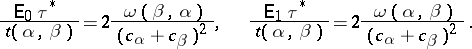 |
Numerical calculations show that for  ,
,
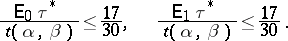 |
In other words, for the values of errors of the first and the second kinds considered, the optimal sequential method of decision between two hypotheses needs approximately half the observations of the optimal method with a fixed number of observations. Moreover, if  , then
 |
References
| [1] | A. Wald, "Sequential analysis" , Wiley (1947) MR0020764 Zbl 0041.26303 Zbl 0029.15805 |
| [2] | A.N. Shiryaev, "Statistical sequential analysis" , Amer. Math. Soc. (1973) (Translated from Russian) MR0445744 MR0293789 Zbl 0267.62039 |
| [3] | A.N. Shiryaev, "Optimal stopping rules" , Springer (1978) (Translated from Russian) MR2374974 MR1317981 MR0445744 MR0293789 MR0283922 Zbl 0391.60002 |
Comments
References
| [a1] | D. Siegmund, "Sequential analysis" , Springer (1985) MR0799155 Zbl 0573.62071 |
| [a2] | R. Lerche, "Boundary crossing of Brownian motion: its relation to the law of the iterated logarithm and to sequential analysis" , Springer (1986) Zbl 0604.62075 |
Sequential analysis. Encyclopedia of Mathematics. URL: http://encyclopediaofmath.org/index.php?title=Sequential_analysis&oldid=23653