Difference between revisions of "Zernike polynomials"
(Importing text file) |
m (gt to >) |
||
| (2 intermediate revisions by one other user not shown) | |||
| Line 1: | Line 1: | ||
| − | + | <!--This article has been texified automatically. Since there was no Nroff source code for this article, | |
| + | the semi-automatic procedure described at https://encyclopediaofmath.org/wiki/User:Maximilian_Janisch/latexlist | ||
| + | was used. | ||
| + | If the TeX and formula formatting is correct and if all png images have been replaced by TeX code, please remove this message and the {{TEX|semi-auto}} category. | ||
| − | + | Out of 61 formulas, 57 were replaced by TEX code.--> | |
| − | + | {{TEX|semi-auto}}{{TEX|part}} | |
| + | Polynomials (cf. also [[Polynomial|Polynomial]]) constructed by F. Zernike [[#References|[a5]]] and by Zernike and H. Brinkman [[#References|[a6]]] for the purpose of approximating certain functions, such as the aberration function of geometrical optics, on the disc $D = \{ ( x , y ) \in \mathbf{R} ^ { 2 } : x ^ { 2 } + y ^ { 2 } \leq 1 \}$. The underlying premise is that errors in circular optical elements can be quantified by mean-square deviation per unit area. Given a function $f$ on $D$ and $n \in \mathbf{N} _ { 0 } = \{ 0,1,2 , \dots \}$, the problem of finding a polynomial $p ( x , y )$ of degree $n$ which minimizes the $L^{2}$-norm | ||
| − | + | \begin{equation*} \| f - p \| _ { 2 } = \left( \int \int _ { D } | f ( x , y ) - p ( x , y ) | ^ { 2 } d x d y \right) ^ { 1 / 2 } \end{equation*} | |
| − | + | is solved by means of orthogonal polynomials (cf. [[Orthogonal polynomials|Orthogonal polynomials]]). This means that for each $n \in \mathbf{N} _ { 0 }$ there is an orthogonal basis for the space $\mathcal{V} _ { n }$ of polynomials of degree $n$, which are orthogonal to each polynomial of lower degree (orthogonality is with respect to the inner product $\langle f , g \rangle = \int \int _ { D } f ( x , y ) \overline { g ( x , y ) } d x d y$). The dimension of $\mathcal{V} _ { n }$ is $n + 1$. In the case of the disc there are at least two useful approaches to constructing orthogonal polynomials, based on the Cartesian or on the polar coordinate system. The Zernike polynomials are associated with the polar coordinate system ($x = r \operatorname { cos } \theta$, $y = r \operatorname { sin } \theta$) and with complex coordinates ($z = x + i y = r e ^ { i \theta }$, $r ^ { 2 } = z \bar{z}$). For $n \in \mathbf{N} _ { 0 }$ and $m = n - 2 j$ with $j = 0 , \dots , n$, the Zernike circle polynomial is | |
| − | + | \begin{equation*} V _ { n } ^ { m } ( x , y ) = e ^ { i m \theta } R _ { n } ^ { m } ( r ), \end{equation*} | |
| − | + | where $R _ { n } ^ { m } ( r )$ is a polynomial of degree $n$ in $r$, of the same parity as $n$. This family has been generalized to "disc polynomials" , associated with the weight function $( 1 - x ^ { 2 } - y ^ { 2 } ) ^ { \alpha } d x d y$ with arbitrary $\alpha > - 1$ (see [[#References|[a3]]]). The formulas will be stated for the general case since they are no more complicated than for the Zernike polynomials ($\alpha = 0$). A convenient indexing is obtained from setting $n = k + l$, $m = k - l$ for arbitrary $k , l \in {\bf N} _ { 0 }$. Then (using the Pochhammer symbol $(a)_ { n } = \prod _ { i = 1 } ^ { n } ( a + i - 1 )$ and the [[Hypergeometric function|hypergeometric function]] $F$), define | |
| + | |||
| + | \begin{equation*} V _ { k + l } ^ { k - l } ( x , y ; \alpha ) = e ^ { i ( k - l ) \theta } R _ { k + l } ^ { k - l } ( r ; \alpha ) = \end{equation*} | ||
| + | |||
| + | \begin{equation*} = \frac { ( \alpha + 1 ) _ { k + l } } { ( \alpha + 1 ) _ { k } ( \alpha + 1 ) _ { l } } z ^ { k } z ^ { l } F \left( - k , - l ; - k - l - \alpha ; \frac { 1 } { z \overline{z} } \right). \end{equation*} | ||
The Zernike radial polynomial is | The Zernike radial polynomial is | ||
| − | + | \begin{equation*} R _ { k + l } ^ { k - l } ( r ; \alpha ) = \end{equation*} | |
| − | + | \begin{equation*} = \frac { ( \alpha + 1 ) _ { k + l } } { ( \alpha + 1 ) _ { k } ( \alpha + 1 ) _ { l } } \sum _ { j = 0 } ^ { \operatorname { min } ( k , l ) } \frac { ( - k ) _ { j } ( - l ) _j} { ( - k - l - \alpha )_j j ! } r ^ { k + l - 2 j }. \end{equation*} | |
| − | The normalization of the polynomials comes from the equation | + | The normalization of the polynomials comes from the equation $V _ { k + l } ^ { k - l } ( 1,0 ; \alpha ) = 1$. The orthogonality relations are |
| − | <table class="eq" style="width:100%;"> <tr><td | + | <table class="eq" style="width:100%;"> <tr><td style="width:94%;text-align:center;" valign="top"><img align="absmiddle" border="0" src="https://www.encyclopediaofmath.org/legacyimages/z/z130/z130080/z13008040.png"/></td> </tr></table> |
| − | <table class="eq" style="width:100%;"> <tr><td | + | <table class="eq" style="width:100%;"> <tr><td style="width:94%;text-align:center;" valign="top"><img align="absmiddle" border="0" src="https://www.encyclopediaofmath.org/legacyimages/z/z130/z130080/z13008041.png"/></td> </tr></table> |
| − | The polynomials can be expressed in terms of [[Jacobi polynomials|Jacobi polynomials]]: for | + | The polynomials can be expressed in terms of [[Jacobi polynomials|Jacobi polynomials]]: for $k \geq l $, |
| − | + | \begin{equation*} R _ { k + l } ^ { k - l } ( r ; \alpha ) = \frac { l ! } { ( \alpha + 1 ) _ { l } } r ^ { k - l } P _ { l } ^ { ( \alpha , k - l ) } ( 2 r ^ { 2 } - 1 ), \end{equation*} | |
and satisfy a Rodrigues formula: | and satisfy a Rodrigues formula: | ||
| − | + | \begin{equation*} V _ { k + l } ^ { k - l } ( x , y ; \alpha ) = \end{equation*} | |
| − | + | \begin{equation*} = \frac { ( - 1 ) ^ { k + l } } { ( \alpha + 1 ) _ { k + l } } ( 1 - z \overline{z} ) ^ { - \alpha } ( \frac { \partial } { \partial z } ) ^ { l } ( \frac { \partial } { \partial \overline{z} } ) ^ { k } ( 1 - z \overline{z} ) ^ { k + l + \alpha }. \end{equation*} | |
| − | The orthogonal polynomials of degree | + | The orthogonal polynomials of degree $n$ (that is, $V _ { n } = \operatorname { span } \left\{ V _ { n } ^ { n - 2 j } : 0 \leq j \leq n \right\}$) satisfy a differential equation: |
| − | + | \begin{equation*} \left( 4 \frac { \partial ^ { 2 } } { \partial z \partial \overline{z} } - \mathcal{D} ^ { 2 } - 2 ( \alpha + 1 ) \mathcal{D} \right) f = \end{equation*} | |
| − | + | \begin{equation*} = - n ( n + 2 + 2 \alpha ) f , \mathcal{D} = z \frac { \partial } { \partial z } + \bar{z} \frac { \partial } { \partial \bar{z} }. \end{equation*} | |
| − | There is an important [[Integral transform|integral transform]] used in the diffraction theory of aberrations (see [[#References|[a1]]], Chap. 9): Let | + | There is an important [[Integral transform|integral transform]] used in the diffraction theory of aberrations (see [[#References|[a1]]], Chap. 9): Let $k , l \in {\bf N} _ { 0 }$, $k \geq l $, and $s>0$, then |
| − | + | \begin{equation*} \int _ { 0 } ^ { 1 } R _ { k + l } ^ { k - l } ( r ; \alpha ) J _ { k - l } ( r s ) ( 1 - r ^ { 2 } ) ^ { \alpha } r d r = \end{equation*} | |
| − | + | \begin{equation*} = \frac { ( - 1 ) ^ { l } } { 2 } \Gamma ( \alpha + 1 ) \left( \frac { 2 } { s } \right) ^ { \alpha + 1 } J _ { k + l + \alpha + 1 } ( s ), \end{equation*} | |
| − | where | + | where $J _ { a }$ denotes the Bessel function of index $a$ (cf. [[Bessel functions|Bessel functions]]). The coefficients of the orthogonal expansion of an aberration function in terms of the Zernike polynomials are related to the so-called primary aberrations (such as astigmatism, coma, distortion), see [[#References|[a1]]], Chap. 5. The disc polynomials for $\alpha \in \mathbf{N} _ { 0 }$ appear as [[Spherical functions|spherical functions]] on the homogeneous spaces $U ( \alpha + 2 ) / U ( \alpha + 1 )$ (where $U$ denotes the unitary group, see [[#References|[a2]]], Vol. 2, Sec. 11.5, pp. 359–363). The Zernike polynomials are key tools in two-dimensional [[Tomography|tomography]]; see [[#References|[a4]]]. |
====References==== | ====References==== | ||
| − | <table>< | + | <table> |
| + | <tr><td valign="top">[a1]</td> <td valign="top"> M. Born, E. Wolf, "Principles of optics" , Pergamon (1965) (Edition: Third)</td></tr><tr><td valign="top">[a2]</td> <td valign="top"> A. Klimyk, N. Vilenkin, "Representations of Lie groups and special functions" , Kluwer Acad. Publ. (1993)</td></tr><tr><td valign="top">[a3]</td> <td valign="top"> T. Koornwinder, "Two-variable analogues of the classical orthogonal polynomials" R. Askey (ed.) , ''Theory and Applications of Special Functions'' , Acad. Press (1975) pp. 435–495</td></tr><tr><td valign="top">[a4]</td> <td valign="top"> R. Marr, "On the reconstruction of a function on a circular domain from a sampling of its line integrals" ''J. Math. Anal. Appl.'' , '''45''' (1974) pp. 357–374</td></tr><tr><td valign="top">[a5]</td> <td valign="top"> F. Zernike, "Beugungstheorie des Schneidensverfahrens und seiner verbesserten Form, der Phasenkontrastmethode" ''Physica'' , '''1''' (1934) pp. 689–704</td></tr><tr><td valign="top">[a6]</td> <td valign="top"> F. Zernike, H. Brinkman, "Hypersphärische Funktionen und die in sphärischen Bereichen orthogonalen Polynome" ''Proc. K. Akad. Wetensch.'' , '''38''' (1935) pp. 161–170</td></tr> | ||
| + | </table> | ||
Latest revision as of 08:49, 10 November 2023
Polynomials (cf. also Polynomial) constructed by F. Zernike [a5] and by Zernike and H. Brinkman [a6] for the purpose of approximating certain functions, such as the aberration function of geometrical optics, on the disc $D = \{ ( x , y ) \in \mathbf{R} ^ { 2 } : x ^ { 2 } + y ^ { 2 } \leq 1 \}$. The underlying premise is that errors in circular optical elements can be quantified by mean-square deviation per unit area. Given a function $f$ on $D$ and $n \in \mathbf{N} _ { 0 } = \{ 0,1,2 , \dots \}$, the problem of finding a polynomial $p ( x , y )$ of degree $n$ which minimizes the $L^{2}$-norm
\begin{equation*} \| f - p \| _ { 2 } = \left( \int \int _ { D } | f ( x , y ) - p ( x , y ) | ^ { 2 } d x d y \right) ^ { 1 / 2 } \end{equation*}
is solved by means of orthogonal polynomials (cf. Orthogonal polynomials). This means that for each $n \in \mathbf{N} _ { 0 }$ there is an orthogonal basis for the space $\mathcal{V} _ { n }$ of polynomials of degree $n$, which are orthogonal to each polynomial of lower degree (orthogonality is with respect to the inner product $\langle f , g \rangle = \int \int _ { D } f ( x , y ) \overline { g ( x , y ) } d x d y$). The dimension of $\mathcal{V} _ { n }$ is $n + 1$. In the case of the disc there are at least two useful approaches to constructing orthogonal polynomials, based on the Cartesian or on the polar coordinate system. The Zernike polynomials are associated with the polar coordinate system ($x = r \operatorname { cos } \theta$, $y = r \operatorname { sin } \theta$) and with complex coordinates ($z = x + i y = r e ^ { i \theta }$, $r ^ { 2 } = z \bar{z}$). For $n \in \mathbf{N} _ { 0 }$ and $m = n - 2 j$ with $j = 0 , \dots , n$, the Zernike circle polynomial is
\begin{equation*} V _ { n } ^ { m } ( x , y ) = e ^ { i m \theta } R _ { n } ^ { m } ( r ), \end{equation*}
where $R _ { n } ^ { m } ( r )$ is a polynomial of degree $n$ in $r$, of the same parity as $n$. This family has been generalized to "disc polynomials" , associated with the weight function $( 1 - x ^ { 2 } - y ^ { 2 } ) ^ { \alpha } d x d y$ with arbitrary $\alpha > - 1$ (see [a3]). The formulas will be stated for the general case since they are no more complicated than for the Zernike polynomials ($\alpha = 0$). A convenient indexing is obtained from setting $n = k + l$, $m = k - l$ for arbitrary $k , l \in {\bf N} _ { 0 }$. Then (using the Pochhammer symbol $(a)_ { n } = \prod _ { i = 1 } ^ { n } ( a + i - 1 )$ and the hypergeometric function $F$), define
\begin{equation*} V _ { k + l } ^ { k - l } ( x , y ; \alpha ) = e ^ { i ( k - l ) \theta } R _ { k + l } ^ { k - l } ( r ; \alpha ) = \end{equation*}
\begin{equation*} = \frac { ( \alpha + 1 ) _ { k + l } } { ( \alpha + 1 ) _ { k } ( \alpha + 1 ) _ { l } } z ^ { k } z ^ { l } F \left( - k , - l ; - k - l - \alpha ; \frac { 1 } { z \overline{z} } \right). \end{equation*}
The Zernike radial polynomial is
\begin{equation*} R _ { k + l } ^ { k - l } ( r ; \alpha ) = \end{equation*}
\begin{equation*} = \frac { ( \alpha + 1 ) _ { k + l } } { ( \alpha + 1 ) _ { k } ( \alpha + 1 ) _ { l } } \sum _ { j = 0 } ^ { \operatorname { min } ( k , l ) } \frac { ( - k ) _ { j } ( - l ) _j} { ( - k - l - \alpha )_j j ! } r ^ { k + l - 2 j }. \end{equation*}
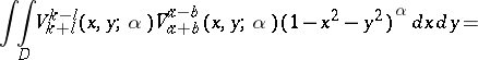
The normalization of the polynomials comes from the equation $V _ { k + l } ^ { k - l } ( 1,0 ; \alpha ) = 1$. The orthogonality relations are
 |
 |
The polynomials can be expressed in terms of Jacobi polynomials: for $k \geq l $,
\begin{equation*} R _ { k + l } ^ { k - l } ( r ; \alpha ) = \frac { l ! } { ( \alpha + 1 ) _ { l } } r ^ { k - l } P _ { l } ^ { ( \alpha , k - l ) } ( 2 r ^ { 2 } - 1 ), \end{equation*}
and satisfy a Rodrigues formula:
\begin{equation*} V _ { k + l } ^ { k - l } ( x , y ; \alpha ) = \end{equation*}
\begin{equation*} = \frac { ( - 1 ) ^ { k + l } } { ( \alpha + 1 ) _ { k + l } } ( 1 - z \overline{z} ) ^ { - \alpha } ( \frac { \partial } { \partial z } ) ^ { l } ( \frac { \partial } { \partial \overline{z} } ) ^ { k } ( 1 - z \overline{z} ) ^ { k + l + \alpha }. \end{equation*}
The orthogonal polynomials of degree $n$ (that is, $V _ { n } = \operatorname { span } \left\{ V _ { n } ^ { n - 2 j } : 0 \leq j \leq n \right\}$) satisfy a differential equation:
\begin{equation*} \left( 4 \frac { \partial ^ { 2 } } { \partial z \partial \overline{z} } - \mathcal{D} ^ { 2 } - 2 ( \alpha + 1 ) \mathcal{D} \right) f = \end{equation*}
\begin{equation*} = - n ( n + 2 + 2 \alpha ) f , \mathcal{D} = z \frac { \partial } { \partial z } + \bar{z} \frac { \partial } { \partial \bar{z} }. \end{equation*}
There is an important integral transform used in the diffraction theory of aberrations (see [a1], Chap. 9): Let $k , l \in {\bf N} _ { 0 }$, $k \geq l $, and $s>0$, then
\begin{equation*} \int _ { 0 } ^ { 1 } R _ { k + l } ^ { k - l } ( r ; \alpha ) J _ { k - l } ( r s ) ( 1 - r ^ { 2 } ) ^ { \alpha } r d r = \end{equation*}
\begin{equation*} = \frac { ( - 1 ) ^ { l } } { 2 } \Gamma ( \alpha + 1 ) \left( \frac { 2 } { s } \right) ^ { \alpha + 1 } J _ { k + l + \alpha + 1 } ( s ), \end{equation*}
where $J _ { a }$ denotes the Bessel function of index $a$ (cf. Bessel functions). The coefficients of the orthogonal expansion of an aberration function in terms of the Zernike polynomials are related to the so-called primary aberrations (such as astigmatism, coma, distortion), see [a1], Chap. 5. The disc polynomials for $\alpha \in \mathbf{N} _ { 0 }$ appear as spherical functions on the homogeneous spaces $U ( \alpha + 2 ) / U ( \alpha + 1 )$ (where $U$ denotes the unitary group, see [a2], Vol. 2, Sec. 11.5, pp. 359–363). The Zernike polynomials are key tools in two-dimensional tomography; see [a4].
References
| [a1] | M. Born, E. Wolf, "Principles of optics" , Pergamon (1965) (Edition: Third) |
| [a2] | A. Klimyk, N. Vilenkin, "Representations of Lie groups and special functions" , Kluwer Acad. Publ. (1993) |
| [a3] | T. Koornwinder, "Two-variable analogues of the classical orthogonal polynomials" R. Askey (ed.) , Theory and Applications of Special Functions , Acad. Press (1975) pp. 435–495 |
| [a4] | R. Marr, "On the reconstruction of a function on a circular domain from a sampling of its line integrals" J. Math. Anal. Appl. , 45 (1974) pp. 357–374 |
| [a5] | F. Zernike, "Beugungstheorie des Schneidensverfahrens und seiner verbesserten Form, der Phasenkontrastmethode" Physica , 1 (1934) pp. 689–704 |
| [a6] | F. Zernike, H. Brinkman, "Hypersphärische Funktionen und die in sphärischen Bereichen orthogonalen Polynome" Proc. K. Akad. Wetensch. , 38 (1935) pp. 161–170 |
Zernike polynomials. Encyclopedia of Mathematics. URL: http://encyclopediaofmath.org/index.php?title=Zernike_polynomials&oldid=17503