Queue with waiting and one service channel
single-server queue
A queue for which the algorithm provides for calls which are not served immediately (having found the system busy) to form a queue; in this connection the service of this call (or batch of calls) can begin only after the service of the previous call (or batch of calls, if the service is in batches) is complete. The basic definitions and notations are to be found in Queue.
The most natural characteristics of the state of a queueing system are the following: a) the waiting time  to the beginning of the service of the
  -th request, and the virtual waiting time
  , which is defined as the time necessary for the system to be free of the calls which arrived up to time
  ; b) the queue length
  at the time of arrival of the
  -th call and the queue length
  at time
  .
.
1) In the "single" case ( ) the values
  are connected by the recurrence relations
 | (1) |
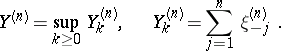
A queueing system in the "multiple" case, when  ,
,  are different from one, may be described by the same type of equation (for the waiting time or queue length). For example, for the queue length
  one has the relation
 | (2) |
where  is the number of calls which can be served during a time
  under continuous operation of the system. If
  ,
,  , then the distribution of
  may be found from the relations
 |
where  is the exponent of the distribution of
  .
.
If one puts  ,
,  , then the solution of (1) has the form
 | (3) |
 |
Hence it follows that if  and
and  for any fixed interval
  as
as  , then there is a limit distribution for the waiting time:
 |
where
 |
Here the variables  are the elements of the sequence
  which extends
  to a sequence which is stationary on the whole line. In what follows it will be assumed that such an extension has been made for all control sequences.
The values
 |
satisfy (1) and have a distribution coinciding with the limit distribution of  . This is the stationary waiting time process.
Let  be ergodic (
 with probability
  ). Then
 |
if  or if
or if  and
and  , where
  . Otherwise
 |
If  , then
 |
if and only if  (the trivial case
  being excluded).
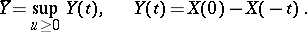
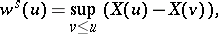
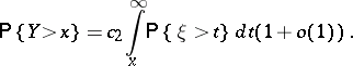
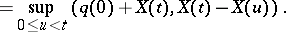
2) As already noted, another possible characteristic of the state of the system is the virtual waiting time  . Roughly speaking, this is the time which the call arriving at time
  would have to wait until the beginning of its service. Let
  be the sum of the service times of the calls which arrive in the system up to time
  , and let
  . An analogue of (3) here is the relation
 | (4) |
Let  be the class of processes with stationary increments in the narrow sense and let
  be the class of processes with independent increments (
 and
and  could here be narrower: for example, it can be supposed that
  is the class of generalized Poisson processes with positive jumps and drift
  ). If the process
  , then it can be extended to a process
  given on the whole line and also in
  . In this case
 |
exists, where
 |
If, in addition,
 |
then the distribution of the process
 |
converges as  to the distribution of the process
 |
which is the strictly stationary virtual waiting time process. Here convergence holds in the strong form:
 |
for any measurable  .
.
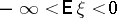
Further, if  and
and  , then
  has a conditional renewal function
  :
:
 |
 |
here
 |
These formulas still hold when  .
.
For systems in which  there are simple relations between the distributions of
  and
and  .
.
3) Ergodic theorems for the queue length can be obtained with the help of the corresponding theorems for the waiting time. For example, let the sequence  be ergodic (metrically transitive). If, in addition,
  , then there is a (stationary) limit distribution for
  such that
 |
If  ,
,  and
and  has a non-lattice distribution, then
 |
 |
where all the components under the probability sign on the right-hand side are independent, and  has a density
 |
 |
If  , then the limit distributions of
  and
and  coincide.
4) If  ,
,  (it is also supposed that
  ,
,  ), then it is possible to obtain an exact formula for the limit distribution of
  :
:
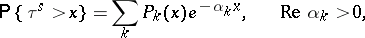
 |
 |
 |
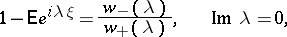
For  and
and  there is the Khinchin–Pollaczek formula for the stationary distribution:
 |
where  is the jump of the process
  (
( if
if  ) and
) and  is the exponent of the distribution of
  .
.
Let  ,
,  be the busy periods of the system (that is, the lengths of the time intervals during which
  ). Then, for the systems considered,
 |
5) For systems in which  (it is also assumed that
  ,
,  ), the distribution of
  coincides with the distribution of the variable
 |
If the distribution of  is known, then the distribution of
  can be found as follows. If
  (this is always true if
  ), then the factorization identity
 |
holds, where  and
and  is the size of the first non-positive sum among
  . This relation permits one to relate
  to the ratio
  in any identity
 | (5) |
in which the functions  admit a representation
 |
( are functions of bounded variation). Equality (5) provides the so-called
  -factorization of the function
  . It explains the following cases, when it is possible to search for
  explicitly.
Assume that  and put
 |
so that  .
.
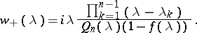
A) If  is a rational function,
  , where
  and
and  are polynomials of degree
  and
and  , respectively, then in the domain
  the function
  has exactly
  zeros
zeros  , and
, and
 |
 |
This means that if the distribution of  can be represented as
 |
where  is a polynomial, then the same type of representation (for other
  and
and  , determined by
  ) also holds for
  .
.
B) If 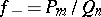 is a rational function, then in the domain
  the function
  has
has  zeros
zeros  , and
, and
 |
In addition to these formulas, giving explicit expressions for the distribution of  , it is also possible, in a broad class of cases, to describe the asymptotic behaviour of
  as
as  . Namely, if
 |
and  , then there is a unique root of the equation
  . In this case, as
  ,
,
 |
If  ,
,  , then
 |
The constants  and
and  have been found explicitly.
Results similar to those discussed in parts 2)–5) are true even for discrete-time systems, when the time  and the random variables of the control sequences take only integer values.
6) Stability theorems investigate conditions under which a small change in the finite-dimensional distributions of the control sequences leads to a small change in the stationary distribution of the waiting time or queue length. The importance of stability for queues is explained by the fact that in real problems various assumptions are usually made on the nature of the control sequences (for example, it is assumed that the  are independent or that the
  are exponentially distributed), whereas, in reality, these assumptions are only approximately satisfied. The question is whether the solution of such "idealized" problems is close to the solution of the actual problem.
To obtain a precise statement of the problem, triangular arrays are used, where equation (1) is controlled by stationary sequences (triangular arrays) 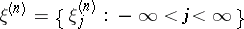 ,
,  . In addition, one considers a stationary sequence
  and puts
 |
The answer to the question posed above is given by the following result.
Let the finite-dimensional distributions of  converge weakly to the corresponding distributions of
  , which is assumed to be ergodic, and let
  . Then for the weak convergence
 | (6) |
(that is, for the convergence of the distributions of the stationary waiting times) it is sufficient that
 |
The stated condition for convergence is almost necessary.
If the control sequences  and
and  are such that
  and
and  are independent and the distributions of
  converge weakly to the distributions of
  , then for (6) it is sufficient that
 |
The situation is similar for the stationary distribution of the virtual waiting time  . If the finite-dimensional distributions of the processes
  converge to the distributions of
  and if the sequence
  is ergodic,
  , then for the convergence of the distributions of
 |
it is sufficient that
 |
7) Asymptotic methods for studying single-server systems (which include stability theorems) give approximate formulas for the case of heavy and light traffic. Let  . Then the system is said to be in heavy traffic conditions if
 |
is close to 0 and in light traffic conditions if  is close to
  .
.
A precise statement, as in part (6), is again related to the introduction of triangular arrays. Specifically, for heavy traffic one considers processes  , depending on a parameter
  . Let
. Let  satisfy the conditions of weak dependence, which guarantee that, as
  ,
,
 |
 |
uniformly in  , where
 |
Then for the stationary virtual waiting time  , as
, as  one has
 |
A similar result holds for the stationary distribution of  .
.
If the condition of heavy traffic is imposed on the sequence  (also in a triangular array relative to the parameter
  ), and it is required that
 | (7) |
then it is also possible to give a fairly complete description of the distribution of the limit waiting time  , including the so-called transition phenomena. Specifically, in addition to (7), let
 |
for any  . Then, if
  as
as  without changing sign, so that
  , then
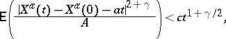
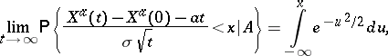
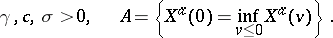
 | (8) |
 |
where  is a standard Wiener process. The value of the right-hand side of (8) can be explicitly calculated. If
  , then
 |
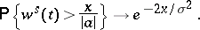
If  ,
,  , then
 |
8) Systems with finite waiting room are characterized as follows: Calls which arrive in the system and find a queue of size  are refused and removed from the system. In this case
  , and the probability
  will be the same as the probability that the
  -th call is refused.
Equation (2) must here be changed to an equation of the form
 |
Let  be metrically transitive. In addition, let the following condition be satisfied: Either
  or
or  and, in the second case,
  cannot be represented in the form
  with
with  . Under these conditions there exists a limit distribution for
  as
as  .
.
If, in addition,  (this holds, for example, when
  and if the remaining control sequences belong to
  ), then it is possible to find an explicit form for the stationary distribution of
  as
as  , since in this case
  is related to a simple homogeneous Markov chain with a finite state space.
There is also a representation for the stationary distribution:
 | (9) |
 |
 |
where  is the position of a particle leaving 0 and wandering with jumps
  ,
,  to the first exit time from the interval
  . If
. If  (that is, if
  ), then the probability (9) can be expressed explicitly in terms of the distributions of
  and
and  .
.
9) In systems with autonomous service, in contrast to the usual queueing system, the service of calls may begin only at the times  where
where  are the elements of a control sequence. Thus, calls which find the system free must wait until the next stage of service.
Side by side with the process  , describing the input stream, one considers the process
  , where
  is defined as the number of calls which would be accepted into service up to time
  if the queue could be infinite. Denoting by
  the length of the queue at time
  , not counting calls in service, and putting
  , one obtains
 |
 |
This equality is similar to (4) and leads to the following result. If the process  is ergodic and
 |
then the distributions of the processes  converge as
  to the distribution of the stationary process
 |
If  or
or  and the remaining control sequences belong to
  , it is possible to give explicit formulas for the distribution of
  .
.
For references see Queueing theory.
Queue with waiting and one service channel. Encyclopedia of Mathematics. URL: http://encyclopediaofmath.org/index.php?title=Queue_with_waiting_and_one_service_channel&oldid=12210