Green function

A function related to integral representations of solutions of boundary value problems for differential equations.

The Green function of a boundary value problem for a linear differential equation is the fundamental solution of this equation satisfying homogeneous boundary conditions. The Green function is the kernel of the integral operator inverse to the differential operator generated by the given differential equation and the homogeneous boundary conditions (cf. Kernel of an integral operator). The Green function yields solutions of the inhomogeneous equation satisfying the homogeneous boundary conditions. Finding the Green function reduces the study of the properties of the differential operator to the study of similar properties of the corresponding integral operator.

Green function for ordinary differential equations.

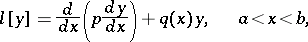
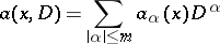
Let be the differential operator generated by the differential polynomial

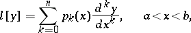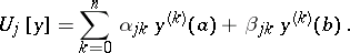
and the boundary conditions , , where

The Green function of is the function that satisfies the following conditions:

1) is continuous and has continuous derivatives with respect to up to order for all values of and in the interval .

2) For any given in the function has uniformly-continuous derivatives of order with respect to in each of the half-intervals and and the derivative of order satisfies the condition

if .

3) In each of the half-intervals and the function , regarded as a function of , satisfies the equation and the boundary conditions , .

If the boundary value problem has trivial solutions only, then has one and only one Green function [1]. For any continuous function on there exists a solution of the boundary value problem , and it can be expressed by the formula

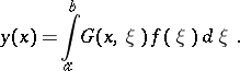If the operator has a Green function , then the adjoint operator also has a Green function, equal to . In particular, if is self-adjoint (), then 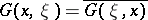, i.e. the Green function is a Hermitian kernel in this case. Thus, the Green function of the self-adjoint second-order operator generated by the differential operator with real coefficients

and the boundary conditions , has the form:

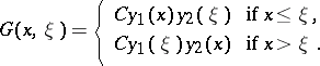Here and are arbitrary independent solutions of the equation satisfying, respectively, the conditions , ; , where is the Wronski determinant (Wronskian) of and . It can be shown that is independent of .

If the operator has a Green function, then the boundary eigen value problem is equivalent to the integral equation 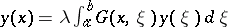, to which Fredholm's theory is applicable (cf. also Fredholm theorems). For this reason the boundary value problem can have at most a countable number of eigen values without finite limit points. The conjugate problem has complex-conjugate eigen values of the same multiplicity. For each that is not an eigen value of it is possible to construct the Green function of the operator , where is the identity operator. The function is a meromorphic function of the parameter ; its poles can be eigen values of only. If the multiplicity of the eigen value is one, then

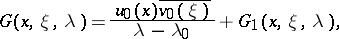where is regular in a neighbourhood of the point , and and are the eigen functions of and corresponding to the eigen values and and normalized so that

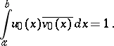If has infinitely-many poles and if these are of the first order only, then there exists a complete biorthogonal system

of eigen functions of and . If the eigen values are numbered in increasing sequence of their absolute values, then the integral

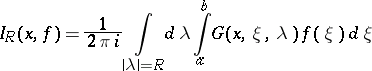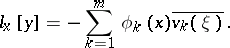
is equal to the partial sum

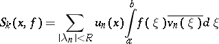of the expansion of with respect to the eigen functions of . The positive number is so selected that the function is regular in on the circle . For a regular boundary value problem and for any piecewise-smooth function in the interval , the equation

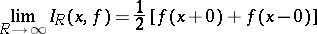is valid, that is, an expansion into a convergent series is possible [1].

If the Green function of the operator has multiple poles, then its principal part is expressed by canonical systems of eigen and adjoint functions of the operators and [2].

In the case considered above, the boundary value problem has no non-trivial solutions. If, on the other hand, such non-trivial solutions exist, a so-called generalized Green function is introduced. Let there exist, e.g., exactly linearly independent solutions of the problem . Then a generalized Green function exists that has properties 1) and 2) of an ordinary Green function, satisfies the boundary conditions as a function of if and, in addition, is a solution of the equation

Here is a system of linearly independent solutions of the adjoint problem , while is an arbitrary system of continuous functions biorthogonal to it. Then

is the solution of the boundary value problem if the function is continuous and satisfies the solvability criterion, i.e. is orthogonal to all .

If is one of the generalized Green functions of , then any other generalized Green function can be represented in the form

where is a complete system of linearly independent solutions of the problem , and are arbitrary continuous functions [3].

Green function for partial differential equations.

1) Elliptic equations. Let be the elliptic differential operator of order generated by the differential polynomial

in a bounded domain and the homogeneous boundary conditions , where are boundary operators with coefficients defined on the boundary of , which is assumed to be sufficiently smooth. A function is said to be a Green function for if, for any fixed , it satisfies the homogeneous boundary conditions and if, regarded as a generalized function, it satisfies the equation

In the case of operators with smooth coefficients and normal boundary conditions, which ensure that the solution of the homogeneous boundary value problem is unique, a Green function exists and the solution of the boundary value problem can be represented in the form (cf. [4])

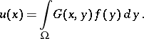In such a case the uniform estimates for ,

are valid for the Green function, and the latter is uniformly bounded if .

The boundary eigen value problem is equivalent to the integral equation

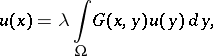to which Fredholm's theory (cf. [5]) is applicable (cf. Fredholm theorems). Here, the Green function of the adjoint boundary value problem is . It follows, in particular, that the number of eigen values is at most countable, and there are no finite limit points; the adjoint boundary value problem has complex-conjugate eigen values of the same multiplicity.

A Green function has been more thoroughly studied for second-order equations, since the nature of the singularity of the fundamental solution can be explicitly written out. Thus, for the Laplace operator the Green function has the form

where is a harmonic function in chosen so that the Green function satisfies the boundary condition.

The Green function of the first boundary value problem for a second-order elliptic operator with smooth coefficients in a domain with Lyapunov-type boundary , makes it possible to express the solution of the problem

in the form

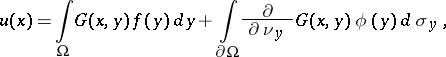where is the derivative along the outward co-normal of the operator and is the surface element on .

If the homogeneous boundary condition has non-trivial solutions, a generalized Green function is introduced, just as for ordinary differential equations. Thus, a generalized Green function, the so-called Neumann function [3], is available for the Laplace operator.

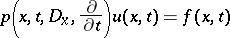
2) Parabolic equations. Let be the parabolic differential operator of order generated by the differential polynomial

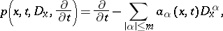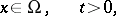and the homogeneous initial and boundary conditions

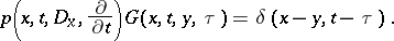
where are boundary operators with coefficients defined for and . The Green function of the operator is a function which for arbitrary fixed with and satisfies the homogeneous boundary conditions and also satisfies the equation

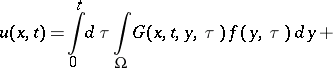
For operators with smooth coefficients and normal boundary conditions, which ensures the uniqueness of the solution of the problem , a Green function exists, and the solution of the equation

satisfying the homogeneous boundary conditions and the initial conditions 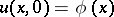, has the form

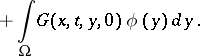In the study of elliptic or parabolic systems the Green function is replaced by the concept of a Green matrix, by means of which solutions of boundary value problems with homogeneous boundary conditions for these systems are expressed as integrals of the products of a Green matrix by the vectors of the right-hand sides and the initial conditions [7].

Green functions are named after G. Green (1828), who was the first to study a special case of such functions in his studies on potential theory.

References

[1]	M.A. Naimark, "Lineare Differentialoperatoren" , Akademie Verlag (1960) (Translated from Russian)
[2]	M.V. Keldysh, "On the characteristic values and characteristic functions of certain classes of non-self-adjoint equations" Dokl. Akad. Nauk. SSSR , 77 : 1 (1951) pp. 11–14 (In Russian)
[3]	V.V. Sobolev, "Course in theoretical astrophysics" , NASA , Washington, D.C. (1969) (Translated from Russian)
[4]	L. Bers, F. John, M. Schechter, "Partial differential equations" , Interscience (1964)
[5]	L. Gårding, "Dirichlet's problem for linear elliptic partial differential equations" Math. Scand. , 1 : 1 (1953) pp. 55–72
[6]	A. Friedman, "Partial differential equations of parabolic type" , Prentice-Hall (1964)
[7]	S.D. Eidel'man, "Parabolic systems" , North-Holland (1969) (Translated from Russian)

References

[a1]	J.K. Hale, "Ordinary differential equations" , Wiley (1980)
[a2]	P.R. Garabedian, "Partial differential equations" , Wiley (1964)

Green function in function theory.

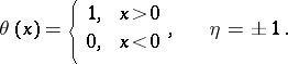
In the theory of functions of a complex variable, a (real) Green function is understood to mean a Green function for the first boundary value problem for the Laplace operator, i.e. a function of the type

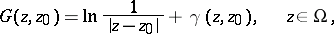(1)

where is the complex variable, is the pole of the Green function, , and is a harmonic function of which takes the values at the boundary . Let the domain be simply-connected and let be the analytic function which realizes the conformal mapping of onto the unit disc so that maps to the centre of the disc, and such that , .

Then

(2)

If is the harmonic function conjugate with , , then the analytic function is said to be a complex Green function of with pole . The inversion of formula (2) yields

(3)

Formulas (2) and (3) show that the problems of constructing a conformal mapping of into the disc and of finding a Green function are equivalent. The Green functions , are invariant under conformal mappings, which may sometimes facilitate their identification (see Mapping method).

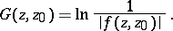
In the theory of Riemann surfaces it is more convenient to define Green functions with the aid of a minimum property, valid for a function (1): Of all functions on a Riemann surface that are positive and harmonic for and have in a neighbourhood of the form

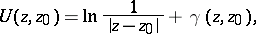(4)

where is a harmonic function which is regular on the entire surface , the Green function, if it exists, is the least, i.e. . Here, the existence of a Green function is typical for Riemann surfaces of hyperbolic type. If a Green function is thus defined, it no longer vanishes, generally speaking, anywhere on the (ideal) boundary of the Riemann surface. The situation is similar in potential theory (see also Potential theory, abstract). For an arbitrary open set , e.g. in the Euclidean space , , the Green function can also be defined with the aid of the minimum property discussed above, but for the expression should be substituted for in formula (4). In general, such a Green function does not necessarily tend to zero as the boundary is approached. A Green function does not exist for Riemann surfaces of parabolic type or for certain domains in (e.g. for ).

References

[1]	S. Stoilov, "The theory of functions of a complex variable" , 1–2 , Moscow (1962) (In Russian; translated from Rumanian)
[2]	R. Nevanlinna, "Uniformisierung" , Springer (1953)
[3]	M. Brélot, "Eléments de la théorie classique du potentiel" , Sorbonne Univ. Centre Doc. Univ. , Paris (1959)

E.D. Solomentsev

Comments

See also [a1] and [a3] for Green functions in classical potential theory, and [a2] for Green functions in axiomatic potential theory.

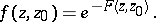
In the theory of functions of several complex variables, more specifically in pluri-potential theory (cf. also Potential theory), Green functions for the complex Monge–Ampère equation have been introduced. Ideally such a Green function should be a fundamental solution for the complex Monge–Ampère operator 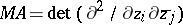, with boundary values and in addition plurisubharmonic (cf. also Plurisubharmonic function). It is only possible to achieve a fair analogy of the classical one-dimensional theory for pseudo-convex domains (cf. Pseudo-convex and pseudo-concave). Several inequivalent definitions of Green function have been proposed. One of these is as follows. Let be a domain in , . Let denote the plurisubharmonic functions (cf. Plurisubharmonic function) on . The Green function for with pole at is

where is a constant depending on . Thus, for every fixed , is plurisubharmonic. For , equals the usual Green function. Of course one wants and also a continuous function to , but this is equivalent to being a hyper-convex domain (that is, a pseudo-convex domain that admits a continuous, bounded plurisubharmonic exhaustion function). If this is the case, one also has:

1) , where is Dirac measure at ,

2) as and is continuous on .

If is strictly convex, then is symmetric: and on . If is only strictly pseudo-convex, then need not be symmetric and not even . One can introduce a kind of Green function in which the symmetry is incorporated, see [a5], but one may loose 1) and 2). For strictly pseudo-convex the following inequality holds (L. Lempert):

with equality for convex domains. Here and denote the Carathéodory and the Kobayashi distance, respectively.

If is a bounded set in , the Green function with pole at for is

and analogous to the one-variable case there is a Robin function

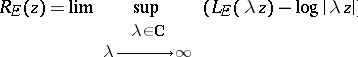and a logarithmic capacity

For general sets , . This capacity has the property that the sets of capacity zero are precisely the pluri-polar sets.

References

[a1]	L.L. Helms, "Introduction to potential theory" , Wiley (Interscience) (1969)
[a2]	K. Janssen, "On the existence of a Green function for harmonic spaces" Math. Annalen , 208 (1974) pp. 295–303
[a3]	N.S. [N.S. Landkov] Landkof, "Foundations of modern potential theory" , Springer (1972) (Translated from Russian)
[a4]	E. Bedford, "Survey of pluri-potential theory" (forthcoming)
[a5]	U. Cegrell, "Capacities in complex analysis" , Vieweg (1988)
[a6]	J.P. Demailly, "Mesures de Monge–Ampère et mesures pluriharmoniques" Math. Z. , 194 (1987) pp. 519–564

Green's function in statistical mechanics.

A time-ordered linear combination of correlation functions (cf. Correlation function in statistical mechanics), which is a convenient intermediate quantity in computations of interacting particles.

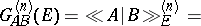
Green's function in statistical quantum mechanics.

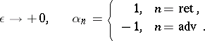
Two-time commutator temperature Green functions are the most often used: retarded , advanced and causal (c). These are defined by the relations:

where

Here, and are time-dependent dynamic variables (operators on the state space of the system in the Heisenberg representation); denotes the average over the Gibbs statistical aggregate; the value of is selected for the sake of convenience. The effectiveness of the use of Green's functions depends to a large extent on the use of spectral representations of their Fourier transforms , . Thus, for non-zero temperature the following representation is valid for the advanced and retarded Green functions:

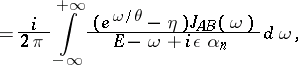Here is the spectral density, , where is the absolute temperature, and is the Boltzmann constant. In the unit system employed, where is the Planck constant. In particular, the following formula is valid:

This formula makes it possible to compute the spectral density (and thus also a number of physical characteristics of the system) by way of a Green's function. Similar spectral formulas also exist for zero temperature. The singularities (poles in the complex plane) of the Fourier transform of a Green function characterize the spectrum and the damping of the elementary perturbations in the system. The principal sources for the computation of a Green function include: a) the approximate solution of an infinite chain of interlacing equations, which is derived directly from the definition of the Green's function by "splitting" the chain on the basis of physical ideas; b) the summation of the physical "fundamental" terms of the series of perturbation theory (summation of diagrams); this method is mainly used in computing causal Green functions and it resembles in many ways the method for the computation of a Green function in quantum field theory.

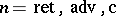
Green's function in classical statistical mechanics

are two-time retarded (ret) and advanced (adv) Green's functions obtained by replacing the operators and in the appropriate quantum formulas established for the quantum case (for ) by the dynamic state functions of the classical system under study, and replacing the commutator (the quantum Poisson brackets) by the classical (ordinary) Poisson brackets; denotes, correspondingly, averaging over Gibbs' classical aggregate. The introduction of a causal Green's function has no meaning here, since the product of the dynamic variables is commutative. In analogy with the quantum case, spectral representations of the Fourier transform of a Green's function exist and can be effectively employed. The principal source for the computation of a classical Green function is the system of equations obtained by infinitesimally varying the Hamiltonian of some system of equations for the correlation functions: the Bogolyubov chain of equations, a system of hydrodynamic equations, etc.

References

[1]	N.N. Bogolyubov, S.V. Tyablikov, "Retarded and advanced Green functions in statistical physics" Soviet Phys. Dokl. , 4 (1960) pp. 589–593 Dokl. Akad. Nauk SSSR , 126 (1959) pp. 53
[2]	D.N. Zubarev, "Double-time Green functions in statistical physics" Soviet Phys. Uspekhi , 3 (1960) pp. 320–345 Uspekhi Fiz. Nauk , 71 (1960) pp. 71–116
[3]	N.N. Bogolyubov, jr., B.I. Sadovnikov, Zh. Eksperim. Teor. Fiz. , 43 : 8 (1962) pp. 677
[4]	N.N. Bogolyubov jr., B.I. Sadovnikov, "Some questions in statistical mechanics" , Moscow (1975) (In Russian)
[5]	, Statistical physics and quantum field theory , Moscow (1973) (In Russian)

V.N. Plechko

Comments

In the special but frequently used case where and are field operators, or creation operators and annihilation operators, one chooses for bosons and for fermions.