Linear system of differential equations with periodic coefficients
A system of  linear ordinary differential equations of the form
 | (1) |
where  is a real variable,
  and
and  are complex-valued functions, and
 | (2) |
The number  is called the period of the coefficients of the system (1). It is convenient to write (1) as one vector equation
 | (3) |
where
 |
It is assumed that the functions  are defined for
  and are measurable and Lebesgue integrable on
  , and that the equalities (2) are satisfied almost-everywhere, that is,
  . A solution of (3) is a vector function
  with absolutely-continuous components such that (3) is satisfied almost-everywhere. Suppose that
  and
and  are an (arbitrarily) given number and vector. A solution
  satisfying the condition
  exists and is uniquely determined. A matrix
  of order
  with absolutely-continuous entries is called the matrizant (or evolution matrix, or transition matrix, or Cauchy matrix) of (3) if almost-everywhere on
  one has
 |
and  , where
  is the unit
  matrix. The transition matrix
  satisfies the relation
 |
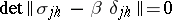
The matrix  is called the monodromy matrix, and its eigen values
  are called the multipliers of (3). The equation
 | (4) |
for the multipliers  is called the characteristic equation of equation (3) (or of the system (1)). To every eigen vector
  of the monodromy matrix with multiplier
  corresponds a solution
  of (3) satisfying the condition
 |
The Floquet–Lyapunov theorem holds: The transition matrix of (3) with  -periodic matrix
  can be represented in the form
 | (5) |
where  is a constant matrix and
  is an absolutely-continuous matrix function, periodic with period
  , non-singular for all
  , and such that
  . Conversely, if
  and
and  are matrices with the given properties, then the matrix (5) is the transition matrix of an equation (3) with
  -periodic matrix
  . The matrix
  , called the indicator matrix, and the matrix function
  in the representation (5) are not uniquely determined. In the case of real coefficients
  in (5),
  is a real matrix, but
  and
and  are complex matrices, generally speaking. For this case there is a refinement of the Floquet–Lyapunov theorem: The transition matrix of (3) with
  -periodic real matrix
  can be represented in the form (5), where
  is a constant real matrix and
  is a real absolutely-continuous matrix function, non-singular for all
  , satisfying the relations
 |
where  is a real matrix such that
 |
In particular, 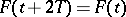 . Conversely, if
  ,
,  and
and  are arbitrary matrices with the given properties, then (5) is the transition matrix of an equation (3) with a
  -periodic real matrix
  .
.
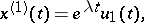
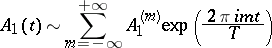
An immediate consequence of (5) is Floquet's theorem, which asserts that equation (3) has a fundamental system of solutions splitting into subsets, each of which has the form
 |
 |
 |
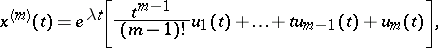 |
where the  are absolutely-continuous
  -periodic (generally speaking, complex-valued) vector functions. (The given subset of solutions corresponds to one
  -cell of the Jordan form of
  .) If all elementary divisors of
  are simple (in particular, if all roots of the characteristic equation (4) are simple), then there is a fundamental system of solutions of the form
 |
Formula (5) implies that (3) is reducible (see Reducible linear system) to the equation
 |
by means of the change of variable  (Lyapunov's theorem).
Let  be the multipliers of equation (3) and let
  be an arbitrary indicator matrix, that is,
 | (6) |
The eigen values  of
of  are called the characteristic exponents (cf. Characteristic exponent) of (3). From (6) one obtains
  ,
,  . The characteristic exponent
  can be defined as the complex number for which (3) has a solution that is representable in the form
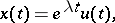 |
where  is a
is a  -periodic vector-valued function. The main properties of the solutions in which one is usually interested in applications are determined by the characteristic exponents or multipliers of the given equation (see the Table).'
<tbody> </tbody>
|
 of all solutions)
 as
as  for any solution)
 )
) -periodic solution
 one has
  (
( is an integer)
 for which
  for all
 one has
  (
( is an integer)
In applications, the coefficients of (1) often depend on parameters; in the parameter space one must distinguish the domains at whose points the solutions of (1) have desired properties (usually these are the first four properties mentioned in the Table, or the fact that  with
with  given). These problems thus reduce to the calculation or estimation of the characteristic exponents (multipliers) of (1).
The equation
 | (7) |
where  and
and  are a measurable
  -periodic matrix function and vector function, respectively, that are Lebesgue integrable on
  (
( ,
,  almost-everywhere), is called an "inhomogeneous linear ordinary differential equation with periodic coefficientsinhomogeneous linear ordinary differential equation with periodic coefficients" . If the corresponding homogeneous equation
 | (8) |
does not have  -periodic solutions, then (7) has a unique
  -periodic solution. It can be determined by the formula
 |
where  and
and  is the transition matrix of the homogeneous equation (8), where
  ,
,  .
.
Suppose that (8) has  linearly independent
  -periodic solutions
  . Then the adjoint equation
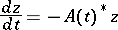 |
also has  linearly independent
  -periodic solutions,
  . The inhomogeneous equation (7) has a
  -periodic solution if and only if that the orthogonality relations
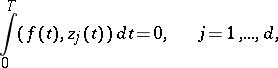 | (9) |
hold. If so, an arbitrary  -periodic solution of (7) has the form
 |
where  are arbitrary numbers and
  is a
is a  -periodic solution of (7). Under the additional conditions
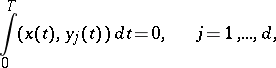 |
the  -periodic solution
  is determined uniquely; moreover, there is a constant
  , independent of
  , such that
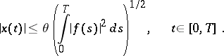 |
Suppose one is given an equation
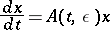 | (10) |
with a matrix coefficient that holomorphically depends on a complex "small" parameter  :
:
 | (11) |
Suppose that for  the series
 |
converges, where
 |
which guarantees the (componentwise) convergence of the series (11) for  in the space
  . Then the transition matrix
  of (10) for fixed
  is an analytic function of
  for
for  . Let
. Let  be a constant matrix with eigen values
  ,
,  . Let
. Let  be the multipliers of equation (10),
  . If
. If  is a multiplier of multiplicity
  , then
 | (12) |
where  are integers. If simple elementary divisors of the monodromy matrix correspond to this multiplier, or, in other words, if to each
  ,
,  , correspond simple elementary divisors of the matrix
  (for example, if all the numbers
  are distinct), then
  is called an
  -fold characteristic exponent (of equation (10) with
  ) of simple type. It turns out that the corresponding
  characteristic exponents of (10) with small
  can be very easily computed to a first approximation. Namely, let
  and
and  be the corresponding normalized eigen vectors of the matrices
  and
and  ;
;
 |
 |
let
 |
be the Fourier series of  , and let
 |
where  are the numbers from (12). Then for the corresponding
  characteristic exponents
  ,
,  , of (10), which become
  for
for  , one has series expansions in fractional powers of
  , starting with terms of the first order:
 | (13) |
Here the  are the roots (written as many times as their multiplicity) of the equation
 |
and  are natural numbers equal to the multiplicities of the corresponding
  (
( ,
,  for
for  ). If the root
  is simple, then
  and the corresponding function
  is analytic for
  . From (13) it follows that cases are possible in which the "unperturbed" (that is, with
  ) system is stable (all the
  are purely imaginary and simple elementary divisors correspond to them), but the "perturbed" system (small
  ) is unstable (
 for at least one
  ). This phenomenon of stability loss for an arbitrary small periodic change of parameters (with time) is called parametric resonance. Similar but more complicated formulas hold for characteristic exponents of non-simple type.
Let  be the distinct multipliers of equation (3) and let
  be their multiplicities, where
 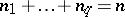 . Suppose that the points
  on the complex
  -plane are surrounded by non-intersecting discs
 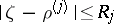 and that a cut, not intersecting these discs, is drawn from the point
  to the point
  . Suppose that with each multiplier
  is associated an arbitrary integer
  and that
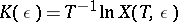
  is the transition matrix of (10). The branches of the logarithm
  are determined by means of the cut. The matrix
  ( "matrix logarithmmatrix logarithm" ) can be defined by the formula
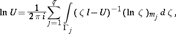 | (14) |
where  is the circle
 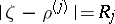 . The set of numbers
  determines a branch of the matrix logarithm. Also,
  for small
  . Generally speaking, formula (14) for all possible
  does not cover all the values of the matrix logarithm, that is, all solutions
  of the equation
  . However, the solution given by (14) has the important property of holomorphy: The entries of the matrix
  in (14) are holomorphic functions of the entries of
  . For equation (10), formula (5) takes the form
 | (15) |
where  ,
,  . If
. If  is determined in accordance with (14), then
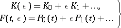 | (16) |
are series that converge for small  . The main information about the behaviour of the solutions as
  which is usually of interest in applications is contained in the indicator matrix
  . Below a method for the asymptotic integration of (10) is given, that is, a method for successively determining the coefficients
  and
and  in (16).
Suppose that  in (11). Although
  , generally speaking there is no branch of the matrix logarithm such that the matrix
  is analytic for
  and
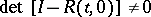
and  . This branch of the logarithm will exist in the so-called non-resonance case, when among the eigen values
  of
of  there are no numbers for which
 |
( is an integer). In the resonance case (when such eigen values exist) equation (10) reduces by a suitable change of variable
  , where
  , to an analogous equation for which the non-resonance case holds. The matrix
  can be determined from the matrix
  .
.
In (16), in the non-resonance case  ,
,  , and the matrices
  ,
,  ,
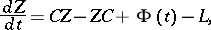
,  are found from the equation
 |
after equating coefficients at the same powers of  in this equation. To determine
  and
and  one obtains a matrix equation of the form
 | (17) |
where  . The matrices
  and
and  are found, and moreover uniquely (the non-resonance case), from (17) and the periodicity condition
  .
.
For special cases of the system (1) see Hamiltonian system, linear and Hill equation.
References
| [1] | I.Z. Shtokalo, "Linear differential equations with variable coefficients: criteria of stability and unstability of their solutions" , Hindushtan Publ. Comp. (1961) (Translated from Russian) |
| [2] | N.P. Erugin, "Linear systems of ordinary differential equations with periodic and quasi-periodic coefficients" , Acad. Press (1966) (Translated from Russian) |
| [3] | V.A. Yakubovich, V.M. Starzhinskii, "Linear differential equations with periodic coefficients" , Wiley (1975) (Translated from Russian) |
Comments
References
| [a1] | R.W. Brockett, "Finite dimensional linear systems" , Wiley (1970) |
| [a2] | J.K. Hale, "Ordinary differential equations" , Wiley (1969) |
Linear system of differential equations with periodic coefficients. Encyclopedia of Mathematics. URL: http://encyclopediaofmath.org/index.php?title=Linear_system_of_differential_equations_with_periodic_coefficients&oldid=16408