Complete problem of eigen values
complete eigen value problem
The problem of calculating all the eigen values (as distinct from the partial problem of eigen values) of a square, usually real or complex, matrix. Often, one has not only to calculate the eigen values but also to construct a basis composed of eigen vectors, or root (principal) vectors, for the matrix.
The solution to the complete problem of eigen values for a matrix  amounts theoretically to constructing the characteristic polynomial
  for this matrix and calculating the, real or complex, roots of it (this makes it impossible to compute the eigen values by a finite computational process). For each eigen value
  , one can determine the corresponding eigen vectors from a homogeneous system of linear equations:
  (
( is the identity matrix). In calculations over the field of complex numbers, a sufficient condition for the existence of a basis of eigen vectors is simplicity of the spectrum, while a necessary and sufficient condition is that the algebraic multiplicity of each eigen value
  (i.e. its multiplicity as a root of the characteristic polynomial
  ) coincides with its geometric multiplicity (i.e. the defect of the matrix
  ). If it is necessary to calculate the root (principal) vectors of multiplicity (degree) exceeding one, one has to consider homogeneous systems of the form
 |
According to this scheme numerical methods of solving the complete problem of eigen values were constructed up to the end of the 1940-s. In the 1930-s, highly effective algorithms (as regards the number of arithmetic operations) were developed for calculating the characteristic polynomial of a matrix in terms of its coefficients. For example, in Danilevskii's method, the computation of the characteristic polynomial for a matrix of order  involves about
  multiplications [1], [2].
Methods in this group have received the name of direct, or exact, ones for the reason that if carried out with exact arithmetic they give the exact values of the coefficients in the characteristic polynomial. The behaviour in real calculations with rounding-off errors could not be tested for problems of any substantial order until digital computers became available. Such tests were carried out in the 1950-s, and as a result, direct methods were completely displaced from numerical practice. There is a catastrophic instability in calculating the eigen values by these methods, and there are two major reasons for this. First, the coefficients in the characteristic polynomial in the majority of exact methods are determined directly or indirectly as components of the solution of a system of linear equations, the matrix of which is built up by columns from the vectors  , where
  is the initial vector in the method. Such a matrix is usually very poorly conditioned, as is evident in particular from the fact that the lengths of the columns are usually very different, and this is the more so the larger
  . Therefore, the coefficients in the characteristic polynomial in general are calculated with very large errors. Secondly, the calculation of the roots of a polynomial is frequently numerically unstable. In that respect, the following example is noteworthy [3]: If in the polynomial
 |
 |
one alters the coefficient of  from
from  to
to  , the perturbed polynomial
  acquires five pairs of complex-conjugate roots; for one of these pairs, the imaginary parts are
  .
.
This sensitivity of the eigen values to perturbations in the coefficients of the characteristic polynomial is usually not accompanied by a comparable sensitivity with respect to the elements of the matrix itself. For example, if this polynomial  is the characteristic polynomial of a symmetric matrix
  , then perturbations of the order of
  in any element in the matrix produce changes at most of the same order in the eigen values.
Modern numerical methods for solving the complete problem of eigen values yield their results without calculating the characteristic polynomial (see Iteration methods). The number of multiplications involved in the best methods is  , where
  is the order of the matrix and
  is a constant independent of
  and having the meaning of the average number of iterations required to calculate one eigen value. The values of
  in the
  algorithm are usually between 1.5 and 2.
Approximate eigen values (vectors) calculated for an ( )-matrix
  by a method
  based on orthogonal transformations can be interpreted as the exact eigen values (vectors) of a perturbed matrix or matrices
  (the
(the  algorithm for matrices of general form, or Jacobi's method or methods based on dividing the spectrum for symmetric and Hermitian matrices are used). Here
  is the equivalent perturbation matrix for the method
  that satisfies bounds of the form
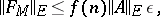 | (1) |
where  is the relative accuracy of the machine arithmetic,
  is the Euclidean matrix norm and
  is a function of the form
  . The number
  has been described above, while the exact values of the constant
  and the exponent
  depend on details of the computation such as the method of rounding-off, the use of scalar-product accumulation, etc. The usual value of
  is 2.
is 2.
The a priori bound (1) allows one to estimate the accuracy in calculating the eigen values (vectors) by the method  . This accuracy depends on the conditioning of the individual eigen values (eigen subspaces).
Let  be a simple eigen value of a matrix
  , let
, let  be the corresponding normalized eigen vector, and let
  be the normalized eigen vector of the transposed matrix
  for the same eigen value. When the matrix
  is perturbed by a matrix
  , the perturbation in the eigen value
  is expressed by the following quantity, accurate up to the second order:
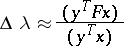 | (2) |
and is estimated as
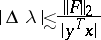 | (3) |
( is the spectral norm). Then the sensitivity of
  to perturbations in the matrix
  is characterized by the number
  , which is called the (individual) condition number of that eigen value. When both vectors
  and
and  are real, the number
  has a simple geometrical meaning: It is the cosine of the angle between
  and
and  , which explains the other name of
  , the distortion coefficient corresponding to
  .
.
If the matrix  is diagonalizable (i.e. has a basis of eigen vectors), then the conditioning of its eigen values
  can be characterized completely. Let
  be the matrix composed by the columns of eigen vectors at
  and having the least condition number among all such matrices. The following theorem applies [4]: All the eigen values of the perturbed matrix
  are enclosed in the region in the complex plane that is the union of the circles
 | (4) |
If this region splits up into connected components, then each of them contains as many eigen values of the perturbed matrix as the number of circles constituting that component (as the norm in (4), one can take the spectral norm, while  can be taken as the spectral condition number).
The number  is called the condition number of the matrix
  in relation to the complete problem of eigen values. Expressed in the spectral norm, it is related to the distortion coefficients as follows:
 |
The perturbation in an eigen vector  related to the simple eigen value
  depends on the perturbation of the matrix
  in a more complicated way. It is determined, generally speaking, not only by the distortion coefficient corresponding to
  but also by those for the other eigen values. The sensitivity of
  also increases if there are eigen values close to
  . In the limiting case where
  becomes a multiple eigen value, it becomes meaningless to consider the sensitivity of an individual eigen vector, and it is necessary to speak of the sensitivity of an eigen (or invariant) subspace.
Qualitatively, the estimates (3) and (4) mean that the perturbations in the eigen values of a diagonalizable matrix  are proportional to the size of the perturbation
  , while the proportionality factors are represented by the condition numbers, individual or global. If the Jordan form of
  is non-diagonal and the eigen value
  corresponds to an elementary divisor
  , then the perturbation of
  in the general case is proportional not to
  , but to
  .
.
The most important particular case of the complete problem of eigen values is to calculate all eigen values (eigen vectors) of a real symmetric or complex Hermitian matrix  . The distortion coefficients for such a matrix are equal to one, and the approximate estimate (3) becomes an exact inequality:
 |
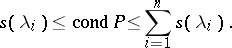
The matrix  in (4) can be taken as orthogonal or unitary, and therefore the global condition number in the spectral norm is equal to one. No matter what the multiplicity of the points in the spectrum of
  , there exists an ordering of the eigen values
  of the matrix
  such that for all
  :
:
 |
Even sharper bounds are possible if not only the matrix  itself is symmetric (Hermitian) but the same applies to the perturbation
  [5].
[5].
In addition, there are some a posteriori estimates for the accuracy of the calculated eigen values and eigen vectors. They are most effective for symmetric and Hermitian matrices  .
.
Let  be an approximate eigen vector and let
  be the exact eigen vector at a simple eigen value
  of the matrix
  . Both vectors are assumed to be normalized. The best estimate of
  that can be obtained by means of the vector
  is given by the value of the Rayleigh functional
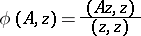 |
corresponding to  , i.e. the number
 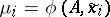 (this applies for any matrix
  , not only Hermitian ones). The vector
 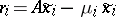 is called the discrepancy vector (or residual).
Let
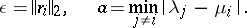 |
A bound for  can readily be derived from the calculated eigen values
  . The following apply:
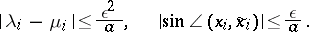 |
If  is a multiple eigen value or if there is a group of eigen values near to
  , it is necessary to estimate the over-all perturbation for the whole group and the perturbation for the corresponding invariant subspace [5].
Along with this ordinary complete eigen value problem, it is often also necessary to solve the so-called generalized eigen value problem:
 | (5) |
In the most important case, the matrices  and
and  are symmetric (Hermitian) and one of them is positive definite. The theory and methods for numerically solving (5) are parallel to those for an ordinary symmetric (Hermitian) eigen value problem.
If neither of the matrices  and
and  is definite or if at least one of them is not symmetric, one uses the
  algorithm [6], which is a generalization of the
  algorithm. Here new effects can occur that are not observed in ordinary complete eigen value problems: infinite eigen values and continuous spectra.
Even more complicated features occur in non-linear eigen value problems:
 |
Such problems are usually solved by reducing them to linear ones of a higher order [7].
References
| [1] | A.M. Danilevskii, Mat. Sb. , 2 : 1 (1937) pp. 169–171 |
| [2] | D.K. Faddeev, V.N. Faddeeva, "Computational methods of linear algebra" , Freeman (1963) (Translated from Russian) |
| [3] | J.H. Wilkinson, "Rounding errors in algebraic processes" , Prentice-Hall (1963) |
| [4] | J.H. Wilkinson, "The algebraic eigenvalue problem" , Oxford Univ. Press (1969) |
| [5] | B.N. Parlett, "The symmetric eigenvalue problem" , Prentice-Hall (1980) |
| [6] | C.B. Moler, G.W. Stewart, "An algorithm for generalized matrix eigenvalue problems" Siam J. Numer. Anal. , 10 (1973) pp. 241–256 |
| [7] | V.N. Kublanovskaya, "Numerical methods of linear algebra" , Novosibirsk (1980) pp. 37–53 (In Russian) |
Comments
In recent years much research has been carried out on the eigen value problem for sparse matrices (cf. Sparse matrix). Because of storage problems, the challenges are even greater here. For the symmetric (Hermitian) case the Lanczos algorithm has proved very successful.
Cf. Iteration methods for a description of the QR algorithm and other iterative algorithms for calculating eigen values.
References
| [a1] | G.H. Golub, C.F. van Loan, "Matrix computations" , North Oxford Acad. (1983) |
Complete problem of eigen values. Encyclopedia of Mathematics. URL: http://encyclopediaofmath.org/index.php?title=Complete_problem_of_eigen_values&oldid=16275