Singular point

A singular point of an analytic function is an obstacle to the analytic continuation of an element of the function of a complex variable along any curve in the -plane.

Let be defined by a Weierstrass element , consisting of a power series

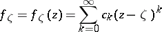(1)

and its disc of convergence

with centre and radius of convergence . Consider all possible curves , i.e. continuous mappings of the interval into the extended complex plane , which begin at the centre of this element , . If the analytic continuation of the given element is possible along any such curve to any point , then the complete analytic function thus obtained reduces to a constant: . For non-trivial analytic functions , the existence of obstacles to the analytic continuation along certain curves is characteristic.

Let be a point in the extended plane on a curve , , , , and on a curve , , , , and let analytic continuation along and to all preceding points , , and , , be possible. Two such curves and are said to be equivalent with respect to the analytic continuation of the given element to the point if there is for any neighbourhood of in a number such that the Weierstrass element obtained from by analytic continuation along to any point , , can be continued along a certain curve located in to an element obtained by continuation along from to any point , .

If analytic continuation to a point is possible along a curve , then it is also possible along all curves of the equivalence class containing . In this case, the pair is said to be regular, or proper; it defines a single-valued regular branch of the analytic function in a neighbourhood of the point.

If analytic continuation along a curve , , , which passes through , , , is possible to all points , , preceding , but is not possible to the point , then is a singular point for analytic continuation of the element along the curve . In this instance it will also be singular for continuation along all curves of the equivalence class which pass through . The pair , consisting of the point and the equivalence class of curves which pass through for each of which is singular, is called a singular point of the analytic function defined by the element . Two singular points and are said to coincide if and if the classes and coincide. The point of the extended complex plane is then called the projection, or -coordinate, of the singular point ; the singular point is also said to lie above the point . In general, several (even a countable set of) different singular and regular pairs obtained through analytic continuation of one and the same element may lie above one and the same point (cf. Branch point).

If the radius of convergence of the initial series (1) , then on the boundary circle of the disc of convergence there lies at least one singular point of the element , i.e. there is a singular point of the analytic function for continuation along the curves , , of the class such that when , . In other words, a singular point of the element is a point such that direct analytic continuation of the element from the disc to any neighbourhood is impossible. In this situation, and generally in all cases where the lack of an obvious description of the class of curves cannot give rise to ambiguity, one usually restricts to the -coordinate of the singular point. The study of the position of singular points of an analytic function, in dependence on the properties of the sequence of coefficients of the initial element , is one of the main directions of research in function theory (see Hadamard theorem on multiplication; Star of a function element, as well as [1], [3], [5]). It is well-known, for example, that the singular points of the series

where , , and is a natural number, fill the whole boundary of its disc of convergence , although the sum of this series is continuous everywhere in the closed disc . Here, is the natural boundary of the analytic function ; analytic continuation of across the boundary of the disc is impossible.

Suppose that in a sufficiently small neighbourhood of a point (or ), analytic continuation along the curves of a specific class is possible to all points other than , for all elements obtained, i.e. along all curves situated in the deleted neighbourhood (respectively, ); the singular point is then called an isolated singular point. If analytic continuation of the elements obtained along the curves of the class along all possible closed curves situated in does not alter these elements, then the isolated singular point is called a single-valued singular point. This type of singular point can be a pole or an essential singular point: If an infinite limit exists when moves towards along the curves of the class , then the single-valued singular point is called a pole (of a function); if no finite or infinite limit exists when moves towards along the curves of the class , then is called an essential singular point; the case of a finite limit corresponds to a regular point . If analytic continuation of the elements obtained along the curves of the class along closed curves surrounding in alters these elements, then the isolated singular point is called a branch point or a many-valued singular point. The class of branch points is in turn subdivided into algebraic branch points and transcendental branch points (including logarithmic branch points, cf. Algebraic branch point; Logarithmic branch point; Transcendental branch point). If after a finite number of single loops around in the same direction within , the elements obtained along the curves of the class take their original form, then is an algebraic branch point and the number is called its order. Conversely, when the loops around give more and more new elements, is a transcendental branch point.

For example, for the function

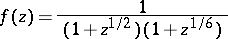the points , (for all curves) are algebraic branch points of order 5. As a point function, can be represented as a single-valued function only on the corresponding Riemann surface , consisting of 6 sheets over joined in a specific way above the points . Moreover, three proper branches of lie above the point , which are single-valued on the three corresponding sheets of ; on one sheet of there is a pole of the second order, and on two sheets of there are poles of the first order. In general, the introduction of the concept of a Riemann surface is particularly convenient and fruitful when studying the character of a singular point.

If the radius of convergence of the initial series (1) , then it represents an entire function , i.e. a function holomorphic in the entire finite plane . When , this function has a single isolated singular point of single-valued character; if is a pole, then is an entire rational function, or a polynomial; if is an essential singular point, then is a transcendental entire function.

A meromorphic function in the finite plane is obtained when analytic continuation of the series (1) leads to a single-valued analytic function in all singular points of which are poles. If is a pole or a regular point, then the total number of poles of in the extended plane is finite and is a rational function. For a transcendental meromorphic function in , the point at infinity can be a limit point of the poles — this is the simplest example of a non-isolated singular point of a single-valued analytic function. A meromorphic function in an arbitrary domain is defined in the same way.

Generally speaking, the projections of non-isolated singular points can form different sets of points in the extended complex plane . In particular, whatever the domain , an analytic function exists in for which is its natural domain of existence, and the boundary is its natural boundary; thus, analytic continuation of the function across the boundary of is impossible. Here, the natural boundary consists of accessible and inaccessible points (see Limit elements). If a point is accessible along the curves of a class (there may be several of these classes), all situated in except for the end point , then only singular points of the function can lie above , since if this were not the case, analytic continuation of across the boundary of through a part of in a neighbourhood of would be possible; the accessible points form a dense set on .

The role of the defining element of an analytic function of several complex variables , , can be played by, for example, a Weierstrass element in the form of a multiple power series

(2)

and the polydisc of convergence of this series

with centre and radius of convergence . By taking in the process of analytic continuation of the element (2) along all possible curves , mappings of the interval into the complex space as basis, a general definition of the singular points , , of the function is obtained, which is formally completely analogous to the one mentioned above for the case .

However, as a result of the overdeterminacy of the Cauchy–Riemann conditions when and the resulting "large power" of analytic continuation, the case differs radically from the case . In particular, for there are domains which cannot be natural domains of existence of any single-valued analytic or holomorphic function. In other words, on specific sections of the boundary of this domain there are no singular points of any holomorphic function defined in , and analytic continuation is possible across them. For example, the Osgood–Brown theorem holds: If a compact set is situated in a bounded domain such that is also a domain, and if a function is holomorphic in , then it can be holomorphically continued onto the whole domain (see also Removable set). The natural domains of existence of holomorphic functions are sometimes called domains of holomorphy (cf. Domain of holomorphy), and are characterized by specific geometric properties. Analytic continuation of a holomorphic function which is originally defined in a domain while retaining its single-valuedness makes it necessary to introduce, generally speaking, many-sheeted domains of holomorphy over , or Riemann domains — analogues of Riemann surfaces (cf. Riemannian domain). In this interpretation, the singular points of a holomorphic function prove to be points of the boundary of its domain of holomorphy . The Osgood–Brown theorem shows that the connected components of cannot form compact sets such that the function is holomorphic in . In particular, for there do not exist isolated singular points of holomorphic functions.

The simplest types of singular points of analytic functions of several complex variables are provided by meromorphic functions in a domain , , which are characterized by the following properties: 1) is holomorphic everywhere in with the exception of a polar set , which consists of singular points; and 2) for any point there are a neighbourhood and a holomorphic function in such that the function can be continued holomorphically to . The singular points are then divided into poles, at which , and points of indeterminacy, at which . In the case of a pole, when moves towards , ; in any neighbourhood of a point of indeterminacy, takes all values . For example, the meromorphic function in has the straight line as its polar set; all points of this straight line are poles, with the exception of the point of indeterminacy . A meromorphic function in its domain of holomorphy can be represented globally in as the quotient of two holomorphic functions, i.e. its polar set is an analytic set.

A point is called a point of meromorphy of a function if is meromorphic in a certain neighbourhood of that point; thus, if a singular point is a point of meromorphy, then it is either a pole or a point of indeterminacy. All singular points of the analytic function which are not points of meromorphy are sometimes called essential singular points. These include, for example, the branch points of , i.e. the branching points of its (many-sheeted) domain of holomorphy . The dimension of the set of all singular points of a holomorphic function is, in general, equal to . Given certain extra restrictions on this set proves to be analytic (and, consequently, is of smaller dimension; see [2]).

References

[1]	A.I. Markushevich, "Theory of functions of a complex variable" , 1–2 , Chelsea (1977) (Translated from Russian)
[2]	B.V. Shabat, "Introduction of complex analysis" , 1–2 , Moscow (1976) (In Russian)
[3]	S. Stoilov, "The theory of functions of a complex variable" , 1–2 , Moscow (1962) (In Russian; translated from Rumanian)
[4]	A. Hurwitz, R. Courant, "Vorlesungen über allgemeine Funktionentheorie und elliptische Funktionen" , 1 , Springer (1964)
[5]	L. Bieberbach, "Analytische Fortsetzung" , Springer (1955) pp. Sect. 3
[6]	L. Bieberbach, "Lehrbuch der Funktionentheorie" , 1–2 , Chelsea, reprint (1945)
[7]	V.S. Vladimirov, "Methods of the theory of functions of several complex variables" , M.I.T. (1966) (Translated from Russian)
[8]	B.A. Fuks, "Introduction to the theory of analytic functions of several complex variables" , Amer. Math. Soc. (1965) (Translated from Russian)
[9]	R.C. Gunning, H. Rossi, "Analytic functions of several complex variables" , Prentice-Hall (1965)
[10]	H. Behnke, P. Thullen, "Theorie der Funktionen meherer komplexer Veränderlichen" , Springer (1970) (Elraged & Revised Edition. Original: 1934)

Comments

Sometimes a point at which an analytic function is not defined but at which it can be defined so as to remain analytic is called a removable singular point.

If , a famous theorem concerning values of an analytic function in a neighbourhood of an essential singular point is Picard's great theorem (cf. Picard theorem). See Fabry theorem for restrictions on the coefficients and powers so that has a singular point.

The Osgood–Brown theorem is also known as the Hartogs extension theorem.

References

[a1]	L. Hörmander, "An introduction to complex analysis in several variables" , North-Holland (1973) pp. Chapt. 2.4
[a2]	H. Cohn, "Conformal mapping on Riemann surfaces" , Dover, reprint (1980)
[a3]	J.B. Conway, "Functions of one complex variable" , Springer (1978)
[a4]	S.G. Krantz, "Function theory of several complex variables" , Wiley (1982) pp. Chapt. 6
[a5]	R.M. Range, "Holomorphic functions and integral representation in several complex variables" , Springer (1986)
[a6]	E.M. Chirka, "Complex analytic sets" , Kluwer (1989) (Translated from Russian)
[a7]	R. Narasimhan, "Several complex variables" , Univ. Chicago Press (1971)
[a8]	R. Remmert, "Funktionentheorie" , 1 , Springer (1984)
[a9]	B. Kaupp, "Holomorphic functions of several variables" , de Gruyter (1983) (Translated from German)

A singular point, or singularity, of an algebraic variety is a point at which smoothness is violated. More accurately, let be an algebraic variety or a scheme of finite type over a field . Then a point is said to be singular if the corresponding local ring is not regular (regularity of a local Noetherian ring with maximal ideal means that ). The set of singular points of is closed in the Zariski topology and is denoted by . If is a reduced variety, then is nowhere dense in . If is an isolated point in , then is said to be an isolated singular point. In order to test whether or not is singular, Jacobi's criterion is used (see Smooth scheme).

A proper birational morphism , where is a smooth variety, is called a resolution of singularities (a desingularization) of the algebraic variety . The existence of a resolution of singularities has been proved for a broad class of varieties, in particular, for all varieties over a field of characteristic (see [13]). As a rule, it is not unique. A resolution of singularities is used to introduce various invariants of a variety ; an example of this are the cohomology spaces . A normal variety for which for all is called a variety with rational singularities. Toroidal singularities [6] and singularities of Schubert varieties [3] are rational. The dimension of the space for an -dimensional variety is called the geometric genus of . See also Resolution of singularities.

The theory of deformations of singularities, i.e. of varieties with singular points, is constructed in parallel with the theory of deformations of (smooth) algebraic varieties. A flat morphism for which for a certain is called a deformation of ; the space is called the base of the deformation. For a variety with an isolated singular point there is a versal deformation which contains all deformations of the variety . The singularity can be rigid, i.e. the base of the versal deformation consists of one point and all its deformations are trivial [4]. The opposite of rigid singular points are smoothable singular points, in the base of the versal deformation of which are points such that are non-singular. The set of points with singular is called the discriminant subset.

An important part in the study of deformations is played by the action of the monodromy group on cohomology spaces of fibres of .

A proper morphism is called a simultaneous resolution of singularities of a family if is a smooth -scheme, and for any the morphism is a resolution of singularities. The versal deformation of simple singular points (see below) permits a simultaneous resolution after a certain finite covering of its base, whereby the Weyl group of the corresponding root system serves as the Galois group of the covering (see [5]).

Singular points of a complex hypersurface.

Let a hypersurface be defined in by one equation , where is a polynomial (or germ of an analytic function at the point ). The ideal in the ring is called the Jacobi ideal of the polynomial ; the singular point 0 is isolated if and only if the space has finite dimension. The dimension of this space is called the Milnor number of the polynomial , and coincides with the rank of the free Abelian group , where is defined by the equation , for small . More precisely, the manifold is homotopically equivalent to a bouquet of spheres of dimension (see [12]). The base of the versal deformation of this singularity is non-singular and is also of dimension (see [9]). The simplest example is a non-degenerate quadratic singularity ; here .

A singularity such that in a deformation only a finite number of other singularities appear is called a simple singular point of the hypersurface [9]; the hypersurface is then defined by one of the following equations:

: , ;

: , ;

: ;

: ;

: .

The lower index is the Milnor number of the singularity. In the case of surfaces these singularities are called Du Val singularities, or rational singular double points. These singular points can also be characterized by the fact that the intersection form on the space is definite. Next, in order of complexity, the unimodal singularities are classified [9]. Natural analogues of these concepts are studied, as well as their connection with catastrophe theory [10]. Many theorems on the singular points of hypersurfaces are extended to the singular points of complete intersections.

Singular points of curves.

Let be the local ring of a singular point of a curve, and let be its normalization; a principal invariant of a singular point is . For an irreducible curve , its arithmetic genus is equal to the geometric genus plus (summation over all singular points of ). Hence, for a plane curve , where is the Milnor number while is the number of branches of the curve at the point .

Let be a plane irreducible curve with a singularity of multiplicity at the point 0 (see Multiplicity of a singular point). then permits a parametrization , , which is written in the form

(a Puiseux expansion). The numbers

are called the characteristic exponents of this expansion, where is the first non-integer exponent in the Puiseux expansion, is the first exponent indivisible by , etc. The sequence , where , is called the characteristic of the singularity. Plane one-dimensional singularities are topologically equivalent if and only if their characteristics coincide (see [8]).

Singular points of surfaces.

Among the resolutions of singularities of normal surfaces, the minimal resolutions through which all remaining resolutions pass, are uniquely distinguished. If is a singular point of a surface , then the curve is said to be exceptional. The weight graph of the curve is a combinatorial invariant of the singular point , and its vertices correspond to the irreducible components of ; the intersection points of the components and are represented by the edges between the corresponding vertices; a weight equal to the genus of the curve , and sometimes even to the index of self-intersection , is attributed to the vertex. The matrix of intersections of components of is negative definite; the graph is connected. The smallest positive divisor such that for all is called the fundamental cycle of the singularity. It always exists and its arithmetic genus

is non-negative. A singular point is rational if and only if ; in this case its multiplicity equals , while the dimension of the tangent Zariski space is greater by one [1]. Elliptic singularities (i.e. singular points with ) are also studied [7].

References

[1]	M. Artin, "On isolated rational singularities of surfaces" Amer. J. Math. , 88 (1966) pp. 129–136
[2]	A. Grothendieck (ed.) et al. (ed.) , Groupes de monodromie en géométrie algébrique. SGA 7 , Lect. notes in math. , 288 , Springer (1972)
[3]	G. Kempf, "On the collapsing of homogeneous bundles" Invent. Math. , 37 (1976) pp. 229–239
[4]	M. Schlessinger, "Rigidity of quotient singularities" Invent. Math. , 14 (1971) pp. 17–26
[5]	H. Pinkham, "Resolution simultanee de points doubles rationnels" M. Demazure (ed.) et al. (ed.) , Sem. sur les Singularités des Surfaces , Lect. notes in math. , 777 , Springer (1980) pp. 179–203
[6]	G. Kempf (ed.) et al. (ed.) , Toroidal embeddings , Lect. notes in math. , 339 , Springer (1973)
[7]	S.S-T. Yau, "On maximally elliptic singularities" Trans. Amer. Math. Soc. , 257 (1980) pp. 269–329
[8]	O. Zariski, "Studies in equisingularity III. Saturation of local rings and equisingularity" Amer. J. Math. , 90 (1968) pp. 961–1023
[9]	V.I. Arnol'd, "Critical points of smooth functions and their normal forms" Russian Math. Surveys , 30 : 5 (1975) pp. 1–75 Uspekhi Mat. Nauk , 30 : 5 (1975) pp. 3–65
[10]	M. Golubitskii, V. Guillemin, "Stable mappings and their singularities" , Springer (1973)
[11]	P.A. Griffiths, J.E. Harris, "Principles of algebraic geometry" , 1–2 , Wiley (Interscience) (1978)
[12]	J. Milnor, "Singular points of complex hypersurfaces" , Princeton Univ. Press (1968)
[13]	H. Hironaka, "Resolution of singularities of an algebraic variety over a field of characteristic zero I, II" Ann. of Math. , 79 (1964) pp. 109–326

V.I. Danilov

Comments

Let the hypersurface in be defined by and let be an isolated singular point. The fibration , where is a small disc of radius around zero, with fibre is called the Milnor fibration.

The ring is the ring of convergent power series in .

The invariant of a singular point on a curve intuitively counts the number of double points concentrated at , [a9].

Let be a polynomial with isolated critical point at . A Morsification of is a polynomial mapping such that (i.e. is a one-dimensional deformation of ) and each has only non-degenerate critical points in a neighbourhood of for small enough . These always exist. Some examples (for ) are as follows, [a6], Sect. 7. Let

: , ;

: , ;

: , ;

: , ,

where in the last two examples is chosen small enough as a function of . For cf. [a6].

It is of course not an accident that the simple hypersurface singularities received the Dynkin diagram labels , , , , . In the examples given above the separatrix diagrams of the Morsifications are in fact the corresponding Dynkin diagrams. (But this is not necessarily the case for every Morsification.) Here the separatrix diagram of consists of the critical points of for some fixed (and a number of lines joining these points (the vertices), where there is a line joining two critical points if and only if there is an integral curve of the gradient vector field

joining these points).

Cf. [8], [a1]–[a7], [a10], [a11] for more material on the interrelations between Dynkin diagrams and singularities and on other occurrences of Dynkin diagrams (the ADE problem).

References

[a1]	V.I. Arnol'd, "Critical points of smooth functions" R. James (ed.) , Proc. Internat. Congress Mathematicians (Vancouver, 1974) , 1 , Canad. Math. Congress (1975) pp. 19–39
[a2]	E. Brieskorn, "Singular elements of semisimple algebraic groups" , Proc. Internat. Congress Mathematicians (Nice, 1970) , 2 , Gauthier-Villars (1971) pp. 279–284
[a3]	E. Brieskorn, "Singularitäten" Jahresber. Deutsch. Math. Verein. , 78 (1976) pp. 93–112
[a4]	S.M. Gusein-Zade, "Dynkin diagrams for singularities of functions of two variables" Funct. Anal. Appl. , 8 : 4 (1974) pp. 295–300 Funkts. Anal. i Prilozh. , 8 : 4 (1974) pp. 23–30
[a5]	S.M. [S.M. Gusein-Zade] Husein-Zade, "The monodromy groups of isolated singularities of hypersurfaces" Russian Math. Surveys , 32 : 2 (1977) pp. 23–65 Uspekhi Mat. Nauk , 32 : 2 (1977)
[a6]	M. Hazewinkel, W. Hesselink, D. Siersma, F.D. Veldkamp, "The ubiquity of Coxeter–Dynkin diagrams" Nieuw Archief voor Wiskunde , 25 (1977) pp. 257–307
[a7]	K. Gawedzki, "Conformal field theory" , Sem. Bourbaki 1988/89 , Exp. 704 , Soc. Math. France (1989) pp. 95–126
[a8]	E. Brieskorn, H. Knörrer, "Plane algebraic curves" , Birkhäuser (1986) (Translated from German)
[a9]	J.-P. Serre, "Groupes algébrique et corps des classes" , Hermann (1959) pp. 65
[a10]	P.J. Slodowy, "Simple singularities and simple algebraic groups" , Lect. notes in math. , 815 , Springer (1980)
[a11]	V.I. Arnol'd, "Singularities of caustics and wave fronts" , Kluwer (1990)

A singular point of a vector field is a point for which . A singular point is isolated if does not vanish at points other than in a sufficiently small neighbourhood of . A singular point is non-degenerate if

A non-degenerate singular point is always isolated.

M.I. Voitsekhovskii

References

[a1]	V.I. Arnol'd, "Singularities of caustics and wave fronts" , Kluwer (1990)

A singular point of a differential equation

(1)

is any point which satisfies the condition

(2)

here are continuous functions in a certain domain . The points of which do not satisfy condition (2) are called the ordinary points of the equation (1). The point is sometimes also called a singular point of the equation (1) if condition (2) is not fulfilled but if the Cauchy problem for equation (1) with initial data has more than one solution.

Equation (1) is a particular case of a system of differential equations in symmetric form:

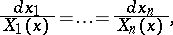(3)

where , and the functions , , are continuous in a domain . A point is called a singular point of the system (3) if , . In the opposite case is an ordinary point of this system.

Let be the set of singular points of the system (3) in the domain . If , then an index and a neighbourhood of the point exist such that the system (3) can be represented in in the normal form

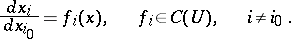Thus, the behaviour of the integral curves of the system (3) in a neighbourhood of an ordinary point is described by theorems of the general theory of ordinary differential equations. In particular, the following parallelizability theorem holds: If through every point of the set passes a unique integral curve of the system (3), then every point of this set has a neighbourhood such that the family of arcs of integral curves of the system (3) which fill is homeomorphic (and if , , diffeomorphic) to a family of parallel straight lines.

If , then no pair exists which possesses the above property, and the integral curves of the system (3) can form different configurations around . Thus, for the equation

where , while the matrix

is non-degenerate, the position of integral curves in a neighbourhood of the point can be of the type of a saddle, a node, a centre, or a focus. The same name is then also given to the point .

The system (3) can be seen as the result of the elimination of the time from an autonomous system of differential equations

(4)

If (4) is a system of class (, uniqueness) in , i.e. , and a unique trajectory of the system passes through every point of the domain , then the points of the set will be stationary points (cf. Equilibrium position) for this trajectory. These points are often called the singular points of this system, insofar as they are (by definition) singular points of the vector field . The integral curves of the system (3) situated in are trajectories of the system (4) other than the stationary positions.

Thus, the problem of the behaviour of integral curves of the system (3) in a neighbourhood of a singular point and the problem of the positioning of the trajectories of the system (4) in a neighbourhood of an equilibrium position are equivalent. Research into these problems follows two main directions.

The first course, which has its origins in the work of H. Poincaré , aims to explain the possible topological types of how the trajectories of the system (4) are situated in a neighbourhood of an isolated stationary point (which can always be considered to coincide with the origin of the coordinates ) and to discover the analytic criteria needed to distinguish them. The most complete results have been obtained for the case where the system (4) can be represented in the form

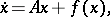(5)

where is a constant non-degenerate matrix and 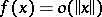when . In this case the point is said to be a simple, or non-degenerate, singular point of the system (4). The following Grobman–Hartman theorem has been established for the system (5): If the matrix does not have purely imaginary eigenvalues, while the function , then there is a homeomorphism of a neighbourhood of the point onto a neighbourhood of the same point which transfers the trajectories of the system (5) to the trajectories of the linear system

(6)

The homeomorphism which realizes a topological correspondence between the trajectories of the systems (5) and (6) is not a diffeomorphism, in general (nor can it be replaced by one).

Under the conditions of this theorem, the stationary point of the system (5) is of the same topological type as the stationary point of the system (6). In particular, for a system of the second order, it will be a saddle if the eigenvalues of the matrix satisfy the condition , and a topological node (node or focus) if (given purely imaginary , the point for the system (6) is a centre, while for the system (5) it is either a centre, a focus or a centre-focus, cf. Centro-focus; Centre and focus problem; Saddle node; Node; Focus).

If the matrix has purely imaginary or zero eigenvalues, then there are, in general, no topological equivalences between the systems (5) and (6) in a neighbourhood of the point . Under these conditions, the behaviour of the trajectories of the system (5) in a neighbourhood of the point has been studied in great detail in those cases where the matrix has at most two eigenvalues with zero real parts while the function is analytic. In particular, for a system of the second order with a non-zero matrix , all possible topological types of positioning of trajectories in a neighbourhood of are clarified, and the coefficient criteria needed to distinguish between them have been given, up to the distinction between a centre and a focus [9]. Here, apart from a saddle, topological node or centre, the point can be a saddle with two separatrices, a saddle-node (a neighbourhood of the point is divided by three trajectories (separatrices) adjoining into three sectors: two hyperbolic sectors, filled by trajectories which leave at both ends, and one parabolic sector, filled by trajectories which leave at one end, while the other approaches ) or a point with elliptical sector (a neighbourhood of this point is divided into 4 sectors: one hyperbolic, two parabolic and one elliptic, filled by trajectories which approach at both ends). For a system of the second order with a zero matrix , algorithms for the resolution of singularities have been worked out (see, for example, Frommer method or local methods in [12]) which, with the aid of a finite number of steps of the resolution process, give a clarification of the topological type of the point , accurate up to the solution of the problem of distinguishing between a centre and a focus. This problem (see Centre and focus problem) arises for a system of the second order in the form (5) when the matrix has purely imaginary eigenvalues, and can arise in the case of two zero eigenvalues of this matrix. It is solved for particular classes of such systems (see, e.g., [14]).

An important characteristic of the isolated stationary point of the system (4) is its Poincaré index. For it is defined as the rotation of the vector field around the point (cf. Rotation of a vector field) along a circle of a sufficiently small radius in the positive direction, measured in units of a complete revolution. For example, the index of a simple saddle is equal to , the index of a node, focus or centre is equal to 1. When is arbitrary, the index of the point is defined as the degree of the mapping (cf. Degree of a mapping) of the sphere of a sufficiently small radius onto itself, defined by the formula:

This course of research has led to the general qualitative theory of differential equations, while the emphasis of the research has shifted from local to global problems — the study of the behaviour of the trajectories of the system (4) in the entire domain , which is taken more and more often as a smooth manifold of some kind.

The other course of research, based on the work of A.M. Lyapunov [2], deals with studies of stability of solutions of systems of the form (4) (especially of equilibrium positions), as well as of non-autonomous systems of differential equations. This research is one of the branches of the theory of stability of motion (see Stability theory).

In complex analysis, the concept of a singular point is introduced for a differential equation

(7)

and also for a system of differential equations

(8)

where is a complex variable, is a rational function in or in the components of the vector , , the coefficients of which are known analytic functions of . Any point of the complex plane which is a singular point of at least one of the coefficients of the function is said to be a singularity for equation (7) (for the system (8)) (see Singular point of an analytic function). Singular points of an equation or system, as a rule, are also singular for their solutions as analytic functions in . They are called fixed singular points (cf. Fixed singular point) of these solutions. Moreover, the solutions of equation (7) (system (8)) can have movable singular points (cf. Movable singular point), the position of which is determined by the initial data of the solution. Studies on various classes of equations of the form (7), (8), aimed at clarifying the analytic nature of the solutions in a neighbourhood of the singular points of the equations, and at clarifying the presence of movable singular points of various types in the solutions of these equations, is the subject of the analytic theory of differential equations.

References

[1a]	H. Poincaré, "Mémoire sur les courbes définiés par une équation differentielle" J. de Math. , 7 (1881) pp. 375–422
[1b]	H. Poincaré, "Mémoire sur les courbes définiés par une équation differentielle" J. de Math. , 8 (1882) pp. 251–296
[1c]	H. Poincaré, "Mémoire sur les courbes définiés par une équation differentielle" J. de Math. , 1 (1885) pp. 167–244
[1d]	H. Poincaré, "Mémoire sur les courbes définiés par une équation differentielle" J. de Math. , 2 (1886) pp. 151–217
[2]	A.M. Lyapunov, "Stability of motion" , Acad. Press (1966) (Translated from Russian)
[3]	V.V. Nemytskii, V.V. Stepanov, "Qualitative theory of differential equations" , Princeton Univ. Press (1960) (Translated from Russian)
[4]	E.A. Coddington, N. Levinson, "Theory of ordinary differential equations" , McGraw-Hill (1955) pp. Chapts. 13–17
[5]	S. Lefschetz, "Differential equations: geometric theory" , Interscience (1957)
[6]	G. Sansone, R. Conti, "Non-linear differential equations" , Pergamon (1964) (Translated from Italian)
[7]	P. Hartman, "Ordinary differential equations" , Birkhäuser (1982)
[8]	V.I. Arnol'd, "Ordinary differential equations" , M.I.T. (1973) (Translated from Russian)
[9]	N.N. Bautin, E.A. Leontovich, "Methods and means for a qualitative investigation of dynamical systems on the plane" , Moscow (1976) (In Russian)
[10]	V.V. Golubev, "Vorlesungen über Differentialgleichungen im Komplexen" , Deutsch. Verlag Wissenschaft. (1958) (Translated from Russian)
[11]	N.P. Erugin, "A reader for a general course in differential equations" , Minsk (1979) (In Russian)
[12]	A.D. [A.D. Bryuno] Bruno, "Local methods in nonlinear differential equations" , Springer (1989) (Translated from Russian)
[13]	A.F. Andreev, "Singular points of differential equations" , Minsk (1979) (In Russian)
[14]	V.V. Amel'kin, N.A. Lukashevich, A.P. Sadovskii, "Non-linear oscillations in second-order systems" , Minsk (1982) (In Russian)

A.F. Andreev

References

[a1]	M.A. Krasnosel'skii, A.I. [A.I. Perov] Perow, A.I. [A.I. Povoloskii] Powolzki, P.P. [P.P. Zabreiko] Sabrejko, "Vektorfelder in der Ebene" , Akademie Verlag (1966) (Translated from Russian)

A singular point of a differentiable mapping is a point which is simultaneously irregular (critical) and improper for . More precisely, let and be two differentiable manifolds of dimensions and , respectively, let be a differentiable mapping of the first onto the second, and let and be local coordinates in them. If the rank of the matrix at a point is equal to , then the mapping is said to be regular at . If the rank of the matrix is equal to at a point , then the mapping is said to be proper at . At a singular point of , the rank of this matrix is not equal to or . See also Singularities of differentiable mappings.

M.I. Voitsekhovskii

A singular point of a real curve is a point at which the first partial derivatives vanish: , . A singular point is called a double point if at least one of the second partial derivatives of the function does not vanish. In studies on the structure of a curve in a neighbourhood of a singular point, the sign of the expression

is studied. If , then the singular point is an isolated point (Fig.a); if , it is a node (or point of self-intersection) (Fig.b); if , then it is either an isolated point or is characterized by the fact that different branches of the curve have a common tangent at this point. If the branches of the curve are situated on different sides of the common tangent and on the same side of the common normal, then the singular point is called a cusp of the first kind (Fig.c); if the branches of the curve are situated on the same side of the common tangent and on the same side of the common normal, then the singular point is called a cusp of the second kind (Fig.d); if the branches are situated on different sides of the common normal and on different sides of the common tangent (Fig.e), or on the same side of the common tangent and on different sides of the common normal (Fig.f), then the singular point is called a point of osculation. See also Double point.

Figure: s085590a

Figure: s085590b

Figure: s085590c

Figure: s085590d

Figure: s085590e

Figure: s085590f

If all partial derivatives of the function up to order inclusive vanish at a certain point and at least one of the derivatives of order differs from zero, then this point is called a singular point of order (a multiple point).

Points which differ in any of their properties from other points of the curve are sometimes called singular points; see, for example, Point of inflection; Point of cessation; Breaking point; Point of rectification; Flat point.

A singular point of a spatial curve defined by the equations , is a point in a neighbourhood of which the rank of the matrix

is less than two.

References

[1]	P.K. Rashevskii, "A course of differential geometry" , Moscow (1956) (In Russian)
[2]	S.S. Byushgens, "Differential geometry" , 1 , Moscow-Leningrad (1940) (In Russian)
[3]	G.M. Fichtenholz, "Differential und Integralrechnung" , 1 , Deutsch. Verlag Wissenschaft. (1964)

A.B. Ivanov

A singular point of a real surface is a point of the surface , , at which the rank of the matrix

is less than two. If the surface is defined as the set of points whose coordinates satisfy an equation , then a point of the surface at which the first partial derivatives of the function vanish is called a singular point:

If not all second partial derivatives of the function vanish at the singular point, then the tangents of the surface at the singular point form a cone. If the tangent cone is non-degenerate, then the singular point is called a conic point; if the cone degenerates to two real planes, then the singular point is called a point of self-intersection of the surface; if the cone is imaginary, then the singular point is an isolated point of the surface.

Singular points can form so-called singular curves of a surface: an edge of regression, lines of self-intersection, lines of osculation, and others.

References

[1]	A.V. Pogorelov, "Differential geometry" , Noordhoff (1959) (Translated from Russian)
[2]	A.P. Norden, "A short course of differential geometry" , Moscow (1958) (In Russian)
[3]	V.A. Il'in, E.G. Poznyak, "Fundamentals of mathematical analysis" , 1–2 , MIR (1982) (Translated from Russian)

A.B. Ivanov

References

[a1]	R.L. Bishop, S.I. Goldberg, "Tensor analysis on manifolds" , Dover, reprint (1980)
[a2]	A. Pollack, "Differential topology" , Prentice-Hall (1974)
[a3]	M. Spivak, "A comprehensive introduction to differential geometry" , 1979 , Publish or Perish pp. 1–5