Elliptic operator

A linear differential or pseudo-differential operator with an invertible principal symbol (see Symbol of an operator).

Let be a differential or pseudo-differential (as a rule, matrix) operator on a domain with principal symbol . If is of order , then is a matrix-valued function on and is positively homogeneous of order in the variable . Then ellipticity means that is an invertible matrix for all , . This concept is called Petrovskii ellipticity.

Another form, Douglis–Nirenberg ellipticity, assumes that is a matrix-valued operator, where is an operator of order , where and are collections of real numbers. Then one can form the matrix of principal symbols , where the function is positively homogeneous in of order . Now Douglis–Nirenberg ellipticity means that the matrix is invertible for all , .

Ellipticity of an operator on a manifold means that the operators obtained from it when it is written in local coordinates are elliptic. Equivalently, this ellipticity can be described as invertibility of the principal symbol , which is a function on , where is the cotangent bundle to and is the same bundle without the zero section. If maps the sections of a vector bundle to the sections of another vector bundle , i.e. , then ellipticity of the operator means invertibility of the linear operator for any point . (Here and are the fibres of and at .) An example of an elliptic operator is the Laplace operator.

Ellipticity of an operator is equivalent to the absence of real characteristic directions. It can also be understood micro-locally. Namely, ellipticity of an operator at a point means invertibility of the matrix (linear transformation) .

Ellipticity of a pseudo-differential operator on a manifold with boundary (for example, an operator from the Boutet de Monvel algebra, [10], [11]) at a boundary point means invertibility of a certain model operator of a boundary value problem on a semi-axis. This model operator is obtained from the original one by straightening the boundary, freezing the principal parts of the operator and the boundary conditions at the point in question, and taking the Fourier transform in the tangential directions (from to ) with subsequent fixing the non-zero vector , which can be regarded as a cotangent vector to the boundary. In the case of a differential operator and differential boundary conditions the condition of ellipticity just described can be expressed in algebraic terms. In this (and sometimes also in a general) case this condition is often called the Shapiro–Lopatinskii condition or the condition of coerciveness.

The most characteristic properties of an elliptic operator are: 1) regularity of the solutions of the corresponding equations; 2) accurate a priori estimates; and 3) the Fredholm property of elliptic operators on compact manifolds.

Henceforth, for simplicity, the coefficients and symbols of all operators are assumed to be infinitely smooth.

Let be an equation, where is an elliptic operator. The simplest regularity property is as follows: If , then . This holds for arbitrary elliptic differential operators with smooth coefficients or arbitrary elliptic pseudo-differential operators (with smooth symbols). It is also true for elliptic operators of a boundary value problem (that is, it is true up to the boundary when the Shapiro–Lopatinskii condition holds). A sharper form of this property is a micro-local version of it: If is an elliptic operator at a point (where is an interior point of ) and , where denotes the wave front (of a distribution or a function), then . Another improvement: If is an elliptic operator of order and , then , where is the Sobolev space, . If is an elliptic differential operator with analytic coefficients and if is analytic, then so is . (In the case of equations with constant coefficients, this property is necessary and sufficient for ellipticity.) The corresponding micro-local version is also valid and can be phrased in the language of analytic wave fronts.

A local a priori estimate for an elliptic operator of order has the form

(1)

where , , , and are two domains in , is a compact part of , in , and the constant does not depend on (but may depend on , , , and ).

A global a priori estimate for an elliptic operator of order on a compact manifold without boundary has the same form as (1), but with and replaced by . In the case of a manifold with boundary one has to take instead of the norm of in (1) norms that take account of the structure of the vector-valued functions and (which contain, generally speaking, boundary components). Suppose, for example, that on a compact manifold with boundary an elliptic operator of the form 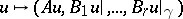has been given, where is an elliptic differential operator of order , the are differential operators of order with , and suppose that the Shapiro–Lopatinskii condition holds (for and the system of boundary operators ). 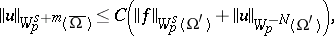Then an a priori estimate in the Sobolev spaces has the form

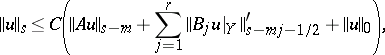where is the norm in , that in , , , and the constant does not depend on (but may depend on , , , , , and the choice of the norm in the Sobolev spaces).

An elliptic operator on a compact manifold (possibly with boundary) determines a Fredholm operator in the corresponding Sobolev spaces, and also in the space of infinitely-differentiable functions. Its index depends only on the principal symbol and does not change under continuous deformations of it. This allows one to raise the problem of calculating the index (see Index formulas).

Elliptic operators with a parameter play an important role (see [12]). When the conditions of ellipticity with a parameter hold on a compact manifold for parameter values of large modulus, then the elliptic operator in question turns out to be invertible, and in the global a priori estimate of the type (1) the last term (the low norm at the right-hand side) can be omitted.

References

[1]	I.G. [I.G. Petrovskii] Petrowski, "Vorlesungen über partielle Differentialgleichungen" , Teubner (1965) (Translated from Russian)
[2]	C. Miranda, "Partial differential equations of elliptic type" , Springer (1970) (Translated from Italian)
[3]	O.A. Ladyzhenskaya, N.N. Ural'tseva, "Linear and quasilinear elliptic equations" , Acad. Press (1968) (Translated from Russian)
[4]	J.L. Lions, E. Magenes, "Non-homogenous boundary value problems and applications" , 1–2 , Springer (1972) (Translated from French)
[5]	L. Bers, F. John, M. Schechter, "Partial differential equations" , Interscience (1964)
[6]	S. Agmon, A. Douglis, L. Nirenberg, "Estimates near the boundary for solutions of elliptic partial differential equations satisfying general boundary conditions" Comm. Pure Appl. Math. , 12 (1959) pp. 623–627
[7]	L. Hörmander, "Linear partial differential equations" , Springer (1963)
[8]	M.A. Shubin, "Pseudo-differential operators and spectral theory" , Springer (1987) (Translated from Russian)
[9]	R.S. Palais, "Seminar on the Atiyah–Singer index theorem" , Princeton Univ. Press (1965)
[10]	B.W. Schulze, "Index theory of elliptic boundary problems" , Akademie Verlag (1982)
[11]	L. Boutet de Monvel, "Boundary problems for pseudo-differential operators" Acta Math. , 126 (1971) pp. 11–51
[12]	M.S. Agranovich, M.I. Vishik, "Elliptic problems with a parameter and parabolic problems of general type" Russian Math. Surveys , 19 (1964) pp. 53–157 Uspekhi Mat. Nauk , 19 : 3 (1964) pp. 53–161

Comments

Boundary value problems for elliptic differential operators can be reduced to systems of pseudo-differential equations on the boundary, the advantage being that the latter is a manifold without boundary. These systems involve the so-called Calderón projection in the space of Cauchy data, this is related to the Hilbert transform in the case of the Cauchy–Riemann operator in the complex plane. Cf. [a1].

[a1] is part of a -volume treatise which grew out of [7].

References

[a1]	L.V. Hörmander, "The analysis of linear partial differential operators" , 3 , Springer (1985)