Lagrange function
A function that is used in the solution of problems on a conditional extremum of functions of several variables and functionals. By means of a Lagrange function one can write down necessary conditions for optimality in problems on a conditional extremum. One does not need to express some variables in terms of others or to take into account the fact that not all variables are independent. The necessary conditions obtained by means of a Lagrange function form a closed system of relations, among the solutions of which the required optimal solution of the problem on a conditional extremum is to be found. A Lagrange function is used in both theoretical questions of linear and non-linear programming and in the construction of certain computational methods.
Suppose, for example, that one has the following problem on a conditional extremum of a function of several variables: Find a maximum or minimum of the function
 | (1) |
under the conditions
 | (2) |
The function  defined by the expression
 | (3) |
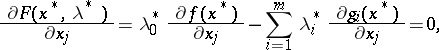
is called the Lagrange function, and the numbers  are called Lagrange multipliers. The following assertion, called the multiplier rule, holds: If
  is a solution of the problem on a conditional extremum (1), (2), then there is at least one non-zero system of Lagrange multipliers
  such that the point
  is a stationary point of the Lagrange function with respect to the variables
  and
and  ,
,  , regarded as independent variables. The necessary conditions for a stationary point of the Lagrange function lead to a system of
  equations,
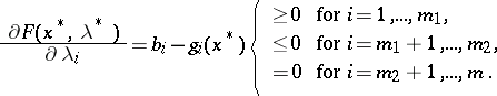
 | (4) |
 |
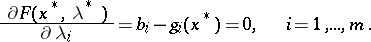 | (5) |
The relations (5) of the resulting system are the conditions (2). The point  gives an ordinary (unconditional) extremum of the Lagrange function
  with respect to
  .
.
For most practical problems the value of  in (3) and (4) can be taken equal to one. However, there are examples (see [1] or [4]) in which the multiplier rule is not satisfied for
  , but is satisfied for
  . To determine conditions that make it possible to distinguish between the cases
  and
and  , one considers (see [2]) the matrices
  and
and  :
:
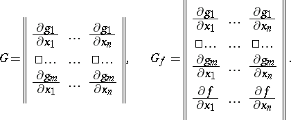 |
Let  be the rank of
  considered at the optimal point
  . If
. If  , then
  ; if
; if  , then in order to satisfy the multiplier rule one must put
  . Moreover, if
  (the case most often occurring in practical problems), then the
  are determined uniquely, but if
  or
or  , then the
  are not determined uniquely. Depending on the case under consideration, one puts
  equal to 0 or 1. Then (4), (5) becomes a system of
  equations with
  unknowns
  ,
,  . It is possible to give an interpretation of the Lagrange multipliers
  that has a definite physical meaning (see Lagrange multipliers).
In the case when the function  to be optimized is quadratic and the conditions (2) are linear, the system of necessary conditions (4), (5) turns out to be linear, and solving it is not difficult. In the general case the system of necessary conditions (4), (5) in the problem on a conditional extremum, obtained by means of a Lagrange function, turns out to be non-linear, and its solution can only be obtained by iterative methods, such as the Newton method. The main difficulty, apart from the computational difficulties of solving a system of non-linear equations, is the problem of obtaining all solutions satisfying the necessary conditions. There is no computational process that ensures that one obtains all solutions of the system (4), (5), and this is one of the restrictions of the application of the method of Lagrange multipliers.
A Lagrange function is used in problems of non-linear programming that differ from the classical problems on a conditional extremum in the presence of constraints of inequality type, as well as of constraints of equality type: Find a minimum or maximum of
 | (6) |
under the conditions
 | (7) |
 | (8) |
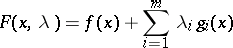
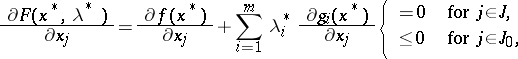
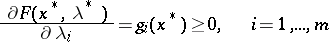
To derive necessary conditions for optimality in the problem (6)–(8) one introduces the Lagrange function
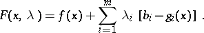 | (9) |
Specifically, consider the case when one looks for a maximum of  . Suppose that
 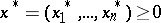 gives a maximum of
  under the restrictions (7), (8), and that the requirement that the restrictions are regular (see [2]) is satisfied at
  ; let
; let  be the set of indices
  from
from  for which
  , let
, let  be the set of indices
  for which
  and let
  be the set of indices
  from
from  for which the restrictions (7) are satisfied at
  as strict inequalities. Then there is a vector
 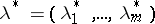 ,
,
 | (10) |
such that
 | (11) |
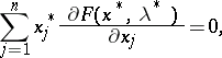
 | (12) |
The necessary conditions stated generalize the conditions (4), (5). Using the concept of a saddle point of the function  , one can interpret these conditions. At a saddle point
  the function
  satisfies the inequalities
 |
A point  at which the conditions (10)–(12) hold satisfies the necessary conditions for the existence of a saddle point of the Lagrange function
  on the set
  and
and  satisfying (10). In the case when
  is concave for
  and
and  is convex if
  and concave if
  ,
,  , the necessary conditions stated turn out to be sufficient, that is, the point
  found from the necessary conditions is a saddle point of the Lagrange function
  for
for  and
and  satisfying (10), and
  is an absolute maximum of
  under the restrictions (7), (8).
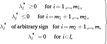
Together with the Lagrange function written in the form (9), one also uses another form of writing a Lagrange function, which differs in the signs of the Lagrange multipliers. The form of writing the necessary conditions also changes. Suppose one is given the following problem of non-linear programming: Find a maximum of
 | (13) |
under the restrictions
 | (14) |
 | (15) |
The restrictions (7) for  reduce to (14) by a simple transformation. The conditions of equality type
  ,
,  , are replaced by the inequalities
 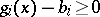 and
and 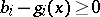 , and they can also be reduced to the form (14).
Suppose that the Lagrange function is written in the form
 | (16) |
and that  is the set of indices
  from
from  for which the restrictions (14) are satisfied as strict inequalities. If
  is the optimal solution of the problem (13)–(15), then if the requirement that the restrictions be regular is satisfied, there is a vector
 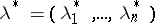 ,
,
 | (17) |
such that
 | (18) |
 | (19) |
(see [2], [3]). Taking into account positive and zero values of  and
and  , one sometimes writes (17)–(19) as follows:
 |
 |
If the restrictions (7) or (14) are linear, then the condition (mentioned above) that the restrictions be regular is always satisfied. Therefore, for linear restrictions the only assumption for the derivation of necessary conditions is that  is differentiable.
If in the problem (13)–(15) the functions  and
and  ,
,  , are concave, then the point
  satisfying the necessary conditions (17)–(19) is a saddle point of the Lagrange function (16) and
  gives an absolute maximum. The fact that the Lagrange function has a saddle point in this case can be proved without any differentiability assumptions on
  and
and  .
.
An analogue of the Lagrange function is used in the calculus of variations in considering problems on a conditional extremum of functionals. Here also it is convenient to write the necessary conditions for optimality in a problem on a conditional extremum as necessary conditions for some functional (the analogue of the Lagrange function) constructed by means of Lagrange multipliers. Suppose, for example, that one is given the Bolza problem: Find a minimum of the functional
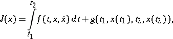 |
 |
in the presence of differential constraints of equality type:
 |
and boundary conditions:
 |
 |
In this conditional extremum problem the necessary conditions are obtained as necessary conditions for an unconditional extremum of the functional (see [4])
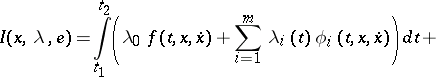 |
 |
formed by means of the Lagrange multipliers
 |
These necessary conditions, which form a closed system of relations for determining an optimal solution  and the corresponding Lagrange multipliers
  and
and  , are written in specific formulations as the Euler equation, the Weierstrass conditions (for a variational extremum) and the transversality condition.
References
| [1] | V.I. Smirnov, "A course of higher mathematics" , 1 , Addison-Wesley (1964) (Translated from Russian) |
| [2] | G.F. Hadley, "Nonlinear and dynamic programming" , Addison-Wesley (1964) |
| [3] | H.W. Kuhn, A.W. Tucker, "Nonlinear programming" , Proc. 2nd Berkeley Symp. Math. Stat. Probab. (1950) , Univ. California Press (1951) pp. 481–492 |
| [4] | G.A. Bliss, "Lectures on the calculus of variations" , Chicago Univ. Press (1947) |
Comments
Since the early 1960's, much effort has gone into the development of a generalized kind of differentiation for extended-real-valued functions on real vector spaces that can serve well in the analysis of problems of optimization. In such problems, which range from models in economics and operations research to variational principles that correspond to partial differential equations, it is often necessary to treat functions that are not differentiable in any traditional two-sided sense and may even have infinite values at some points. See [a2].
References
| [a1] | R.T. Rockafellar, "Convex analysis" , Princeton Univ. Press (1970) |
| [a2] | R.T. Rockafellar, "The theory of subgradients and its applications to problems of optimization. Convex and nonconvex functions" , Heldermann (1981) |
| [a3] | M. Avriel, "Nonlinear programming: analysis and methods" , Prentice-Hall (1976) |
| [a4] | L. Cesari, "Optimization - Theory and applications" , Springer (1983) |
| [a5] | N.I. Akhiezer, "The calculus of variations" , Blaisdell (1962) (Translated from Russian) |
Lagrange function. Encyclopedia of Mathematics. URL: http://encyclopediaofmath.org/index.php?title=Lagrange_function&oldid=13134