Frobenius method
This method enables one to compute a fundamental system of solutions for a holomorphic differential equation near a regular singular point (cf. also Singular point).
Suppose one is given a linear differential operator
 | (a1) |
where for  and some
  , the functions
 | (a2) |
are holomorphic for  and
and  (cf. also Analytic function). The point
  is called a regular singular point of
  . Formula (a1) gives the differential operator in its Frobenius normal form if
  .
.
The Frobenius method is useful for calculating a fundamental system for the homogeneous linear differential equation
 | (a3) |
in the domain  near the regular singular point at
  . Here,
  , and for an equation in normal form, actually
  . The cut along some ray is introduced because the solutions
  are expected to have an essential singularity at
  .
.
The Frobenius method is a generalization of the treatment of the simpler Euler–Cauchy equation
 | (a4) |
where the differential operator  is made from (a1) by retaining only the leading terms. The Euler–Cauchy equation can be solved by taking the guess
  with unknown parameter
  . One gets
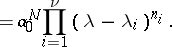
  with the indicial polynomial
 | (a5) |
 |
In the following, the zeros  of the indicial polynomial will be ordered by requiring
 |
It is assumed that all  roots are different and one denotes their multiplicities by
  .
.
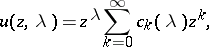
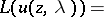
The method of Frobenius starts with the guess
 | (a6) |
with an undetermined parameter  . The coefficients
  have to be calculated by requiring that
 | (a7) |
This requirement leads to  and
and
 | (a8) |
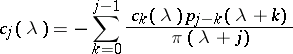
as a recursion formula for  for all
  . Here,
  are polynomials in
  of degree at most
  , which are given below.
The easy generic case occurs if the indicial polynomial has only simple zeros and their differences  are never integer valued. Under these assumptions, the
  functions
 |
are a fundamental system of solutions of (a3).
Complications.
Complications can arise if the generic assumption made above is not satisfied. Putting  in (a6), obtaining solutions of (a3) can be impossible because of poles of the coefficients
  . These solutions are rational functions of
  with possible poles at the poles of
  as well as at
  .
.
The poles are compensated for by multiplying  at first with powers of
  and differentiation by the parameter
  before setting
  .
.
Since the general situation is rather complex, two special cases are given first. Let  denote the set of natural numbers starting at
  (i.e., excluding
  ). Note that neither of the special cases below does exclude the simple generic case above.
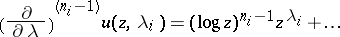
All solutions have expansions of the form
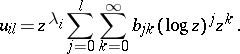 |
The leading term  is useful as a marker for the different solutions. Because for
  and
and  , all leading terms are different, the method of Frobenius does indeed yield a fundamental system of
  linearly independent solutions of the differential equation (a3).
Special case 1.
For any  , the zero
  of the indicial polynomial has multiplicity
  , but none of the numbers
  is a natural number.
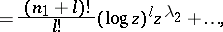
In this case, the functions
 |
 |
 |
are  linearly independent solutions of the differential equation (a3).
Special case 2.
Suppose  .
.
Then the functions
 |
 |
all with  and
and 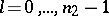 , are
, are  linearly independent solutions of the differential equation (a3). The solution for
  may contain logarithmic terms in the higher powers, starting with
  .
.
Special case 3.
Let  and let
  be a zero of the indicial polynomial of multiplicity
  for
for  .
.
In this case, define  to be the sum of those multiplicities for which
  . Hence,
 |
The functions
 |
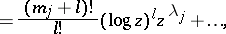 |
with  and
and  , are
, are  linearly independent solutions of the differential equation (a3).
The method looks simpler in the most common case of a differential operator
 | (a9) |
Here, one has to to assume that  to obtain a regular singular point. The indicial polynomial is simply
 |
 |
Only two special cases can occur:
1)  . The functions
 |
 |
are a fundamental system.
2)  . The functions
 |
 |
with  in the second function, are two linearly independent solutions of the differential equation (a9). The second solution can contain logarithmic terms in the higher powers starting with
  .
.
The Frobenius method has been used very successfully to develop a theory of analytic differential equations, especially for the equations of Fuchsian type, where all singular points assumed to be regular (cf. also Fuchsian equation). A similar method of solution can be used for matrix equations of the first order, too. An adaption of the Frobenius method to non-linear problems is restricted to exceptional cases. The approach does produce special separatrix-type solutions for the Emden–Fowler equation, where the non-linear term contains only powers.
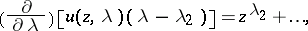
Computation of the polynomials  .
.
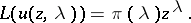
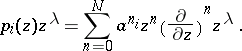
In the guess
 |
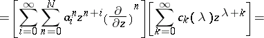
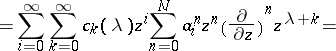
the coefficients  have to be calculated from the requirement (a7). Indeed (a1) and (a2) imply
 |
 |
 |
 |
 |
 |
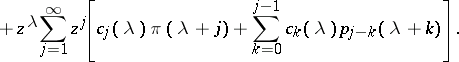 |
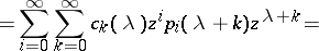
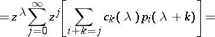
Here,  are polynomials of degree at most
  determined by setting
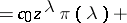
 |
Because of (a7), one finds  and the recursion formula (a8).
References
| [a1] | R. Redheffer, "Differential equations, theory and applications" , Jones and Bartlett (1991) |
| [a2] | F. Rothe, "A variant of Frobenius' method for the Emden–Fowler equation" Applicable Anal. , 66 (1997) pp. 217–245 |
| [a3] | D. Zwillinger, "Handbook of differential equations" , Acad. Press (1989) |
Frobenius method. Encyclopedia of Mathematics. URL: http://encyclopediaofmath.org/index.php?title=Frobenius_method&oldid=12220